I walk the (train) line - part trois - Dijkstra’s revenge

(TL;DR: Author algorithmically confirms what he already knows - that there is a way to get from Newtown Station to a tasty burger. Shortest path from Newtown to tasty burger discovered. Author can’t stop thinking about cheeseburgers. Why didn’t he choose a gym as his destination?)

This is part three of our epic: here is part one, and here is part two.

Now for some unfinished business: back to OpenStreetMap

We have so far:

• gathered some OpenStreetMap (OSM) data, and
• we have subset this data for a region containing Newtown Station and Small Bar (where some tasty burgers await us), and
• we have plotted our map using our pretty_graph() function, and
• we have learnt about breadth-first search, but have not applied it to our map.

Here is our map of interest:

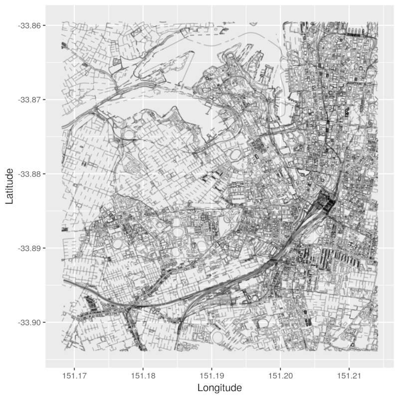
We want to convert this into a graph so that we can apply our breadth-first search algorithm from the last post to it.

What information do we need to apply our breadth-first search? All we need are edges and nodes! Let’s take a look at how many nodes there are in our OSM data:

length(unique(osm_data_subset$nodes$attrs$id))

## [1] 85126

How many ways?

length(osm_data_subset$ways$attrs$id)

## [1] 16212

These numbers feel a little bit too high. Our OSM data may contain information about nodes that are not associated with any way in our dataset. Let’s investigate!

Reading the valuable OpenStreetMap wiki page describing OSM Elements, we find that this may in fact be the case:

Nodes can be used to define standalone point features. For example, a node could represent a park bench or a water well.

As the running time of our breath-first-search algorithm depends on the number of nodes and edges in our graph, we could speed it up by applying it only to the relevant nodes and edges. There’s no sense in applying our algorithm to an edge that makes up part of a river, or to the nodes that represent water wells. I cannot walk on water, nor am I interested in water wells!

How can we reduce the number of elements in our dataset to speed up our algorithm?

Let’s learn some more about the OpenStreetMap data model.

The OSM data model - hierarchical, it is

Here are the definitions of nodes, ways and relations taken from here:

A node represents a specific point on the earth’s surface defined by its latitude and longitude. Each node comprises at least an id number and a pair of coordinates.

A way is an ordered list of between 2 and 2,000 nodes that define a polyline. Ways are used to represent linear features such as rivers and roads.

A relation is a multi-purpose data structure that documents a relationship between two or more data elements (nodes, ways, and/or other relations).

If we were to depict the above definitions in a graph-like structure, it would looks like this:

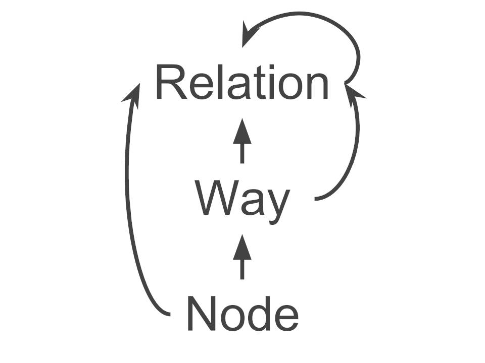
There are two functions from the osmar package that let us traverse this hierarchy. These are find_up() and find_down().

find_*() them elements!

According to the osmar documentation for find_up() and find_down(), this is what they do:

For a given ID these functions return all IDs of related elements.

Relations, ways and nodes have IDs in our dataset. We are good to proceed.

find_up()

According to the previous visualisation, nodes are at the bottom of our hierarchy. So by passing one or more node IDs into find_up(), the function returns the associated way IDs and relation IDs, if any. For ways, we can return associated way IDs and relation IDs, if any. As relations can be made up of other relations, we return associated relation IDs, if any.

find_down()

This is the inverse of the above. I’m sure you can figure this one out!

Putting it all together

This is what we will do:

1. Get all the relevant way IDs in our osmar object. We are only interested in road-like ways (remember, ways include things like rivers and wells). So we will keep ways that have a key, k, equal to ‘highway’. According to this OSM wiki page, highways identify any kind of road, street or path. So we will get ourselves a vector of highway-way IDs.
2. We will use find_down() on these way IDs to return a list of the highway-way IDs and the node IDs that make up those highway-ways.
3. We will then use the subset() function on the full osmar object that we started with to return a reduced osmar object containing the nodes and ways that we are interested in.
4. Our original Newtown Station and Small Bar nodes can’t be found in the set of nodes that make up the ways in our graph as they are landmarks that don’t fall neatly on any ‘way’. We will find the nearest nodes to Newtown Station and Small Bar that are related to some ‘way’ as a proxy for our source and destination nodes.
5. We will then convert our OSM subset into an igraph object.
6. Convert our graph into an adjacency list.

We will then have all that is required to apply our breadth-first search algorithm to our adjacency list!

Steps 1 through to 3 - subsetting the data

Boom!

highways <- find(osm_data_subset, way(tags(k == 'highway')))
highways_nodes <- find_down(osm_data_subset, way(highways))
osmar_highways_and_nodes <- subset(osm_data_subset, ids = highways_nodes)

Let’s take a look at our reduced osmar object:

print(osmar_highways_and_nodes)

## osmar object
## 28965 nodes, 6580 ways, 0 relations

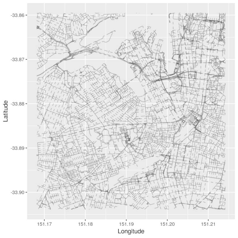
Yes! We started out with 85,126 nodes. We are now down to 28,965. We started out with 16,212 ways and are now down to 6,580 ways. If we plot the reduced map, we can see that it looks a lot sparser!

pretty_graph(osmar_highways_and_nodes, edge_alpha = 0.2)

Step 4 - finding the nearest node in a way

These are our original source and destination node IDs.

newtown_station <- '4735625743'
small_bar <- '1346628719'

I won’t go into much detail here. Here is a little function named find_pedestrian_node which calls osmar's find_nearest_node function and returns the nearest node included in a highway-way that is also a pedestrian-way. Here it is in full. It can also be found in the repo.

find_pedestrian_node <- function(osm_data, node) {
  node <- find_nearest_node(osm_data, node(node), way(tags(k == "highway" & v == "pedestrian")))
  nearest_highway_node <- subset(osm_data, node_ids = node)
  return(nearest_highway_node)
}

Let’s apply it!

nearest_to_newtown <- find_pedestrian_node(osm_data_subset, newtown_station)
nearest_to_small_bar <- find_pedestrian_node(osm_data_subset, small_bar)
print(nearest_to_newtown$nodes$attrs$id)

## [1] 3891123785

print(nearest_to_small_bar$nodes$attrs$id)

## [1] 1427601758

Step 5 - convert our data into a graph using igraph

igraph is an open source graph analysis package written in C. It contains a bunch of useful tools to convert our data structures into different representations of graphs (such as the adjacency list representation from part two of this series). The R port of this package interfaces with igraph's C library so it should generally be faster than the low-level R code that we’ve written thus far!

library(igraph)

One of the suggested packages listed on osmar’s CRAN entry is igraph. One reason for this is that the osmar package contains a function that easily converts our osmar object into an igraph object!

osmar's as_igraph function

Converting our osmar object into an igraph object is simple. Let’s use osmar’s as_igraph function:

igraph_highways_and_nodes <- as_igraph(osmar_highways_and_nodes) %>%
  as.undirected()

Let’s check its class.

class(igraph_highways_and_nodes)

## [1] "igraph"

Woohoo! Now that we’ve got ourselves an igraph object, we can use some handy igraph functions on our graph. For example, let’s get the number of vertices in our graph:

vcount(igraph_highways_and_nodes)

## [1] 19004

What about the number of edges?:

ecount(igraph_highways_and_nodes)

## [1] 22356

But wait a minute…why do we have only 19,004 nodes in our graph when our original osmar object contains 28,965 nodes?

I have an answer for you! Remember that ways are collections of nodes? Our subset osmar object contains ways that refer to nodes that fall outside of our map’s perimeter. For example, way id 3188239 is made up of 9 nodes. Only one of those nodes falls within our map’s perimeter!

If you’re interested in how to debug issues like this, follow me down the rabbit hole in the next section. Otherwise, skip to the next section.

Sidenote - using the OpenStreetMap API to get details of nodes outside of our map subset

The latest version of the OSM API is detailed here. Here is how you can use it to get the details of any node, way or relation by ID.

1. Navigate to the OSM website.
2. Open up Chrome developer tools.

3. Make sure you’re on the ‘Console’ tab. We’ll be writing some JavaScript here!

   

4. We’ll be making a call to the API. According to the API specification, we can get an XML response by making a call of this format: GET /api/0.6/[node|way|relation]/#id. So we will be making a GET request, which will take one of the following three forms:

• /api/0.6/node/<node_id> to get details of the
• /api/0.6/way/<way_id> to get details of the
• /api/0.6/relation/<relation_id> to get the details of the

I’m going to pick node ID 2240223186 which is part of way ID 3188239. I already know that this node falls outside of our subset map. Let’s get its details using some JavaScript! Type this in the Chrome Console:

var httpRequest = new XMLHttpRequest();
httpRequest.open('GET', '/api/0.6/node/2240223186');
httpRequest.send();

If all goes well, we can checkout our our XML reponse like this:

httpRequest.responseText;

Which should print something like this:

<?xml version="1.0" encoding="UTF-8"?>
<osm version="0.6" generator="CGImap 0.6.1 (11637 thorn-03.openstreetmap.org)" copyright="OpenStreetMap and contributors" attribution="http://www.openstreetmap.org/copyright" license="http://opendatacommons.org/licenses/odbl/1-0/">
 <node id="2240223186" visible="true" version="2" changeset="19370313" timestamp="2013-12-10T04:07:03Z" user="mrpulley" uid="67896" lat="-33.8671718" lon="151.2167234"/>
</osm>

We can use the lat and lon attributes in our response to search for this node in the OpenStreetMap search box:

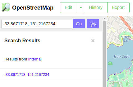
This is where the node is:

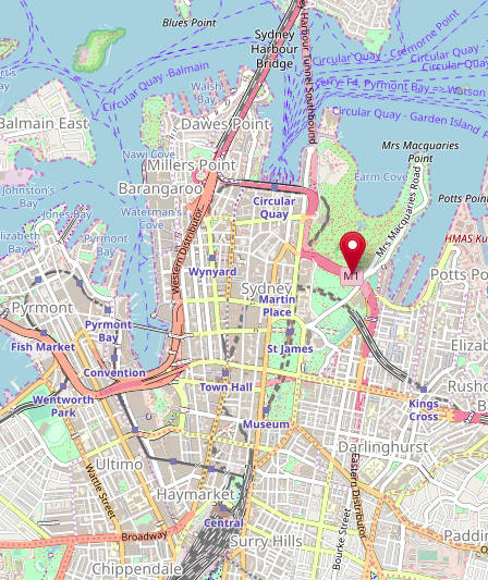
And we can see that it sits just outside of our map perimeter!

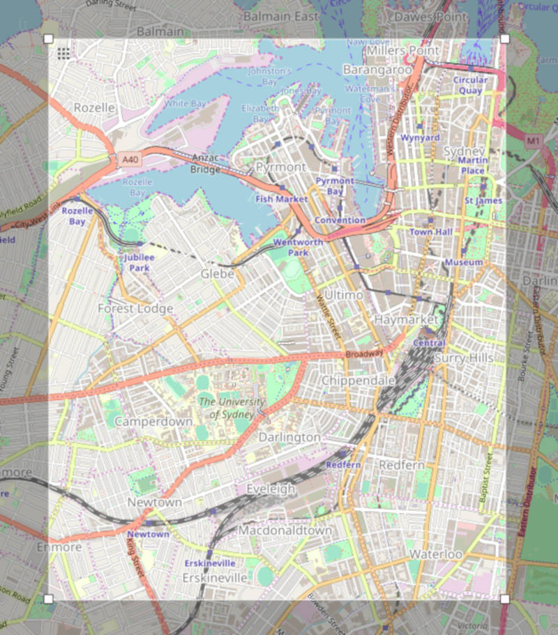
We have survived our quest and have returned home stronger.

Step 6 - convert our graph into an adjacency list

We know how to make an adjacency list using low-level code from part two. Now that you know how adjacency lists work, we can be lazy and use igraph's as_adj_list function!

adj_list_highways_and_nodes <- igraph_highways_and_nodes %>%
  as_adj_list()

The resulting adjacency list is a R list object.

class(adj_list_highways_and_nodes)

## [1] "list"

The list element names are the node IDs!

names(adj_list_highways_and_nodes) %>%
  head(10)

##  [1] "20827842"   "3814697125" "2869677788" "1810713242" "8965944"   
##  [6] "33683546"   "1826240863" "1826240636" "8410958"    "8408936"

If we index into a node in our list, we can apply the name function to get our adjacent nodes. Let’s use our source node as an example:

adj_list_highways_and_nodes[['3891123785']] %>%
  names()

## [1] "3891123784" "3891123778"

It’s breadth-first search time!

I will source the breadth-first search function from last time. It can be found here.

source('breadth_first_search.R')

bfs_path <- breadth_first_search(adj_list_highways_and_nodes, nearest_to_newtown, nearest_to_small_bar)
head(bfs_path, 10)

##  [1] "3891123785" "3891123778" "6128173386" "3891123774" "1843636548"
##  [6] "3123414079" "1833285840" "5802864448" "3123414075" "1840727738"

Success! We have some nodes on our path!

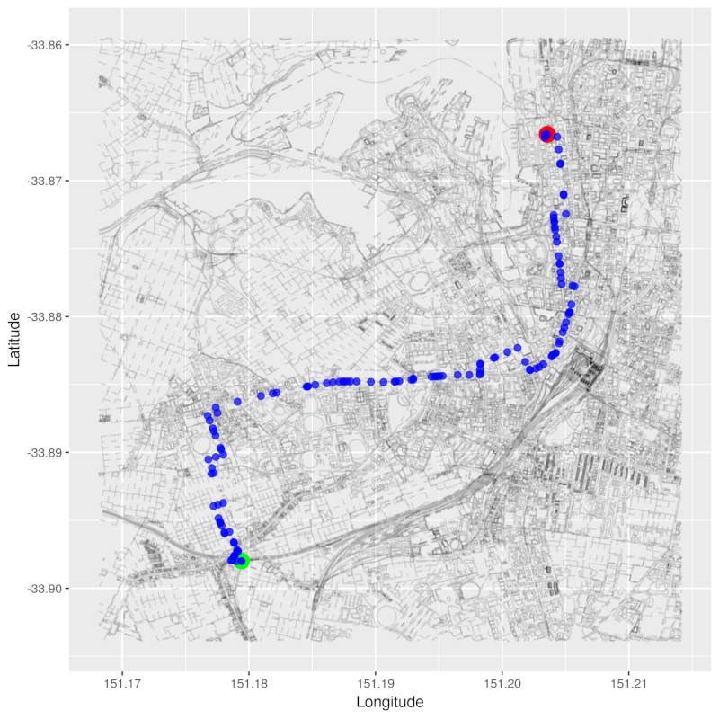
Is there a path from Newtown to Small Bar?

Yes! Of course a path exists from Newtown Station to Small Bar.

pretty_graph(osm_data_subset, nearest_to_newtown, nearest_to_small_bar,
             path_nodes = bfs_path,  node_alpha = 0.7, edge_alpha = 0.1)

What is the path’s length?

I will be using my function get_path_lengths to get our path’s distance in kilometres. It can be found here.

source('get_path_length.R')

bfs_distance_in_kms <- get_path_length(bfs_path, igraph_highways_and_nodes)
print(bfs_distance_in_kms)

## [1] 6.554328

~6.5 kms…but Google Maps says:

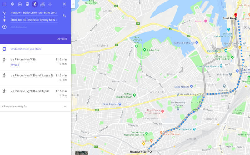
NOOOOOOOOOOOOOOOOOOOOOOOOOOOOOOOOOOOOOOOOOOOOOOOOOO!

With BFS, we have shown the existance of a path, which is an easier condition to satisfy than finding the shortest path from our source to destination. Let’s tackle this trickier problem.

Is this the shortest path?

According to Google Maps, there is a shorter path. Therefore, our path is not the shortest path!

Introducing Dijkstra’s algorithm

Dijkstra’s algorithm is a famous algorithm which was created by Dutch computer scientist Edsger Dijkstra. It is a solution to the single-source shortest path problem for graphs with non-negative edge weights. Single-source means that the algorithm solves for the shortest paths from a single source node to all other nodes in our graph. In our case, we’re really only interested in the shortest path from our source node (Newtown Station), to our destination node (Small Bar). But the output of Dijkstra will give us the shortest path from Newtown Station to every other node in our graph! Exciting!

Here is my implementation in (R-like) pseudo code.

dijkstra(graph_representation, source_node) {
  # input:
  #   - some graph represented as a weighted adjacency list or matrix
  #   - source node ID
  # output:
  #   - vec of distances of shortest paths from all nodes in graph to source node
  #   - vec of predecessors of nodes on shortests paths

  LARGE_DISTANCE = 999999

  vec_of_distances = vector of all node IDs in graph initialised with LARGE_DISTANCE
  vec_of_distances[source_node] = 0

  vec_of_predecessors = vector of all node IDs initialised to NA
  vec_of_predecessors[source_node] = source_node

  vec_of_nodes_to_process = vector of all node IDs in graph

  while nodes_left_to_process(vec_of_nodes_to_process) {
    min_distance_node = node with smallest distance in vec_of_distances
    min_distance = distance to min_distance_node

    for each adjacent_node to min_dist_node  {
        distance_from_adj_to_min_dist = distance from adjacent node to min_distance_node
      known_dist_to_adj_node = currently known distance to adjacent node from vec_of_distances

      # if the distance to the adjacent node is smaller if we go via the min_distance_node...
        if min_distance + distance_from_adj_to_min_dist < known_dist_to_adj_node {
          # set the distance to the adjacent node to the new, smaller distance via the min dist node
          vec_of_distances[adjacent_node] = min_distance + distance_from_adj_to_min_dist
          # set the predecessor to the adjacent node as the min dist node
          vec_of_predecessors[adjacent_node] = min_distance_node
        }
    }
    # we are done processing the min_dist_node so remove it from vec_of_nodes_to_process
    remove_min_dist_node(vec_of_nodes_to_process)
  }
}

Let’s break this down!

Input: some representation of a weighted graph

Previously, we cared about the existence of a path. The lengths of the edges on the path didn’t matter. All we wanted to know was whether we could get from one point of the graph to another. This time, we are trying to answer a more complex problem. We want to know the answer to this question:

Of all the paths from the source node to the destination node, which is the shortest?

To answer this question, we need to know the edge weights (in this case, the lengths of edges between nodes, in metres. osmar's as_igraph function creates estimates of these edge weights for us in this line by calling distHaversine from the geosphere package like so:

weights <- distHaversine(x[from, c("lon", "lat")], x[to, c("lon", "lat")])

So it turns out that we already have our weights in our igraph_highways_and_nodes object! To find out about the haversine formula, see this awesome page!

Let’s create ourselves a weighted adjacency list. I couldn’t find a way to do it using the osmar and igraph packages so here is my implementation.

Initialise!

There are a few things we need to do before we can get to the loops that are at the heart of Dijkstra.

What is the LARGE_DISTANCE constant and vec_of_distances?

The type of graph search we are going to use in Dijkstra is a priority-first search. This implies that we will be processing our nodes in some specific order by some definition of priority.

So what is our definition of priority? We want to process nodes in order of distance from our source node, where those closest to our source node are processed before those that are further away.

Let’s compare this to our breadth-first search algorithm from the previous post. Here, we started with our source node and processed each node adjacent to it in some arbitrary order (in this case, the order they happened to appear in our data!). We paid no attention to edge weights. We added each adjacent node to the end of our queue (again, in some arbitrary order). Then we procesed the node at the front of our queue. Et cetera, et cetera, et cetera! So it follows that if all edge weights in are graph are equal, Dijkstra becomes a breath-first search algorithm as we lose the ability to prioritise nodes by distance from our source node!

To make our algorithm process nodes in order of distance from our source node, we create a vector of node distances, where the names attribute of our distances vector contains node IDs. We initialise all our distances to some extremelly large number (or infinity). We then find our source node in our distances vector, and set its distance value to zero. This ensures that When we ask the question “Of all the nodes left to process, which has the smallest distance from our source node?” in our first iteration of our while loop, we start at our source node!

Here is a slice of our distances vector immediately after its initialisation:

What is vec_of_predecessors?

We create another vector of all the nodes in our graph. But this time, the values of our vector will be the predecessor of the node along the currently known minimum distance path. Once our algorithm has finished running, we’ll use this to recover our shortest path in the same way as we did in the last post for BFS.

In this case, we initialise all values with NAs. Here’s a slice of our predecessors vector:

What is vec_of_nodes_to_process?

This one is easy! This is a vector of all the node IDs in our graph. It’ll be used to keep track of which nodes are yet to be processed in our graph.

Time to get loopy

while….

While we still have nodes left…

find the min_distance_node

Here, we find the node with the currently known smallest distance from our source node in our distances vector. This is where we find which node to prioritise in our priority-first search!

and for each adjacent node…

We now know which node to prioritise. We will then go through each node adjacent to our min_distance_node in no particular order and compare some distances.

perform edge relaxation

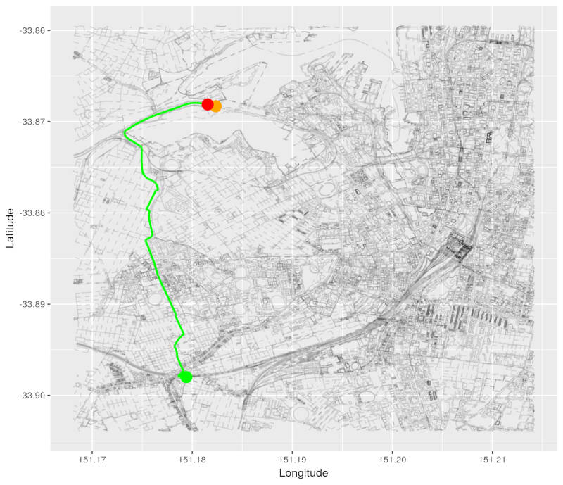
What the hell is edge relaxation? I will explain this visually using one of the many iterations of our while loop.

We have 2 coloured nodes in the below graph:

1. Green - our source node (Newtown Station).
2. Red - our minimum distance node. Of all our nodes that haven’t been processed yet, this one has the smallest distance from our source node.

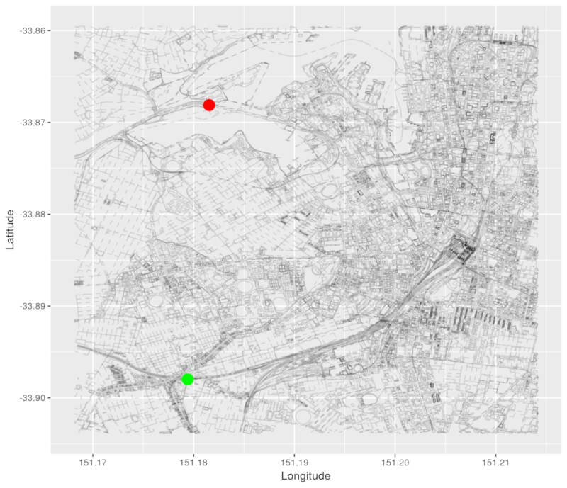
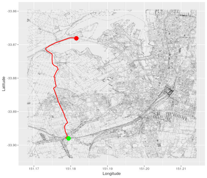
Here is the path from our source node to our minimum distance node.

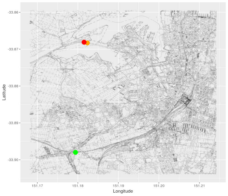
We then start processing nodes adjacent to our minimum distance node. Our adjacent node is coloured in orange:

Here is the currently known path from our source node to the adjacent node.

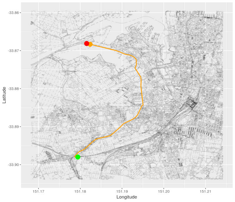
We can clearly see that this path is longer than the path to our minimum distance node! We can get to the adjacent node via the minimum distance node in a shorter distance than via the orange path.

How can we check for shorter ways to get to our adjacent node using some code? In our pseudocode, we have the following inequality:

if min_distance + distance_from_adj_to_min_dist < known_dist_to_adj_node

Here is a description of each variable:

• min_distance = the length of the path from source to the minimum distance node that is currently being processed (i.e. the length of the red path).
• distance_from_adj_to_min_dist = the weight of the direct edge (i.e. the distance) from our minimum distance node to our adjacent node.
• known_dist_to_adj_node = the length of the currently known path from our source node to our adjacent node (i.e. our orange path).

In other words, if the length of the minimum distance path plus the incremental edge length from the minimum distance node to the adjacent node is less than the currently known path to the adjacent node, we can lower the cost (i.e. distance) of getting to the adjacent node by going via the minimum distance node.

Edge relaxation is defined by these lines:

if min_distance + distance_from_adj_to_min_dist < known_dist_to_adj_node

> vec_of_distances[adjacent_node] = min_distance + distance_from_adj_to_min_dist
> vec_of_predecessors[adjacent_node] = min_distance_node

We have established that we can get to the adjacent node via the minimum distance node in a shorter distance than that of the currently known path to the adjacent node. So we simply update our vector of distances and vector of predecessors to reflect our finding!

This new path via the minimum distance node is coloured in green in this graph:

Then remove min_distance_node from vec_of_nodes_to_process

Once all nodes adjacent to the minimum distance node have been processed, we remove it from the vector of nodes that are left to process.

NEXT!

While we still have nodes left to process, we take the one with the currently known minimum distance and continue until we run out of nodes!

Dijkstra time!

Let’s do this! Here is my implementation of Dijkstra.

source('dijkstra.R')

Execute!

results <- dijkstra_shortest_path(igraph_highways_and_nodes, nearest_to_newtown, nearest_to_small_bar)

In the following, satisfying-to-watch video, the minimum distance nodes are coloured in blue. You will see orange circles jumping around our graph - these are the adjacent nodes affected by edge relaxation!

The results are in…

Here is our shortest path:

pretty_graph(osm_data_subset, nearest_to_newtown, nearest_to_small_bar,
             path_nodes = results$path,  node_alpha = 0.7, edge_alpha = 0.1)

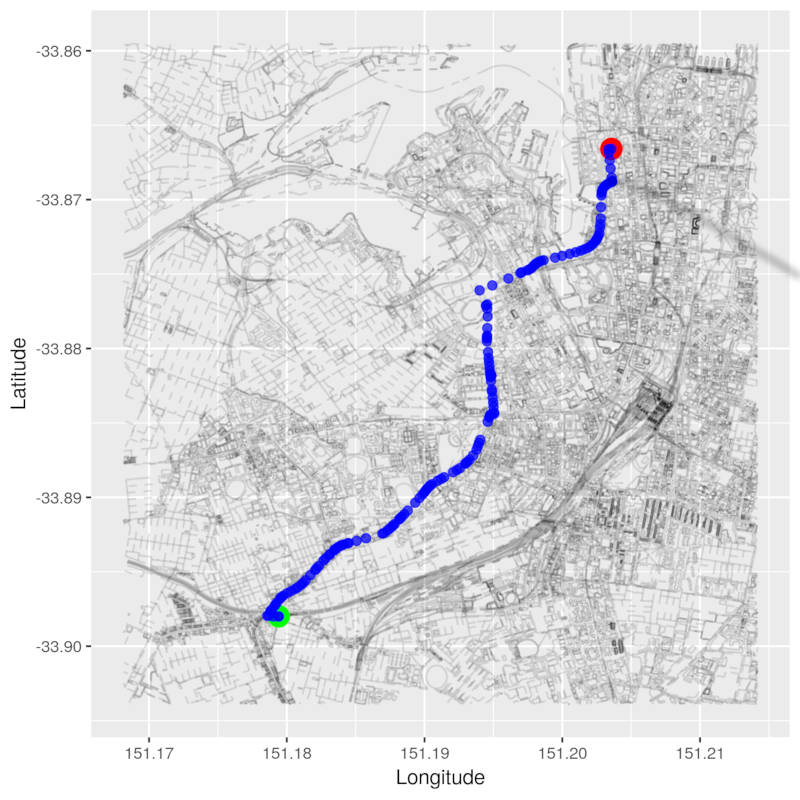
And here is its length:

distances_dijkstra <- results$distances
results$distances[get_node_id(nearest_to_small_bar)]/1000

## 1427601758
##   4.877405

pretty_graph(osm_data_subset, nearest_to_newtown, nearest_to_small_bar,
             path_nodes = results$path,  node_alpha = 0.7, edge_alpha = 0.1)

~4.9 kms! That’s more like it!!!

What have we learnt?

• OSM data is hierarchical
• The igraph package contains some useful functions to help us work with graphs
• We ran breadth-first search on our map after we converted it to an adjacency list
• We learnt about the OSM API
• We learnt about the details of Dijkstra’s algorithm and wrote a low level implementation of it

Next time…

In the final (I promise!) post in this series, we will cover a few things.

• Why does Dijkstra work? It’s time to get mathematical!
• Unfortunately, the shortest path turns out to be a boring path to walk. Our original problem was to come up with (reasonable and interesting) new paths to walk to work. We will figure out a way to accomplish this.

Justin