(Trying) to get to the top of R-bloggers emails

23 minute read

(TL;DR: Author analyses R-Bloggers emails using Gmail API. Decides on when to post to get to the top of the email list. This could either work well or fail spectacularly if he’s missed something. Either way, he learnt a lot. Let’s take a chance!

I have never been at or towards the top of R-Bloggers’ daily emails.

R-bloggers emails display posts in descending order by posted date. The most recent posts are found at the top. I want to find out these things:

When are these emails sent?
What’s the time difference between the post listed at the top and the date these emails are sent?
When should I make my post so that it will closer to the top of these emails?

Let’s get going!

Where the data at? - gmailr

I use Gmail. So my choice is simple - use the gmailr package!

Some prework - enabling the Gmail API

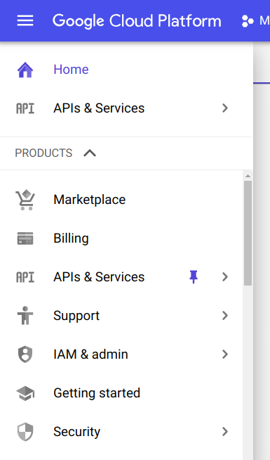
First, navigate to the Google Cloud Platform console and sign in.

Once you’re logged in, expand the menu bar in the top left corner of the page. Look for APIs & Services and click on it!

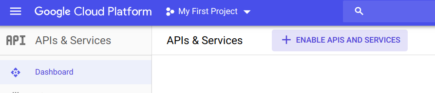
Now click on ENABLE APIS AND SERVICES.

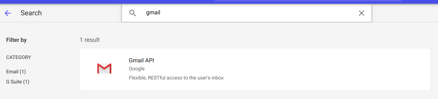
Search for the Gmail API and click on the result.

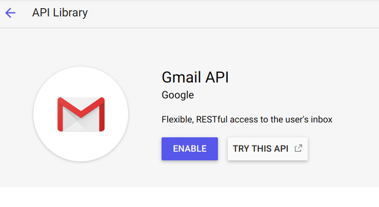
If you’re cool with it, click the ENABLE button.

Click on the Create credentials button and then on OAuth client ID.

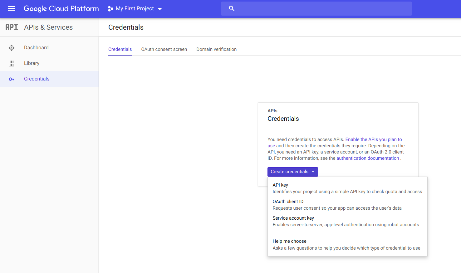
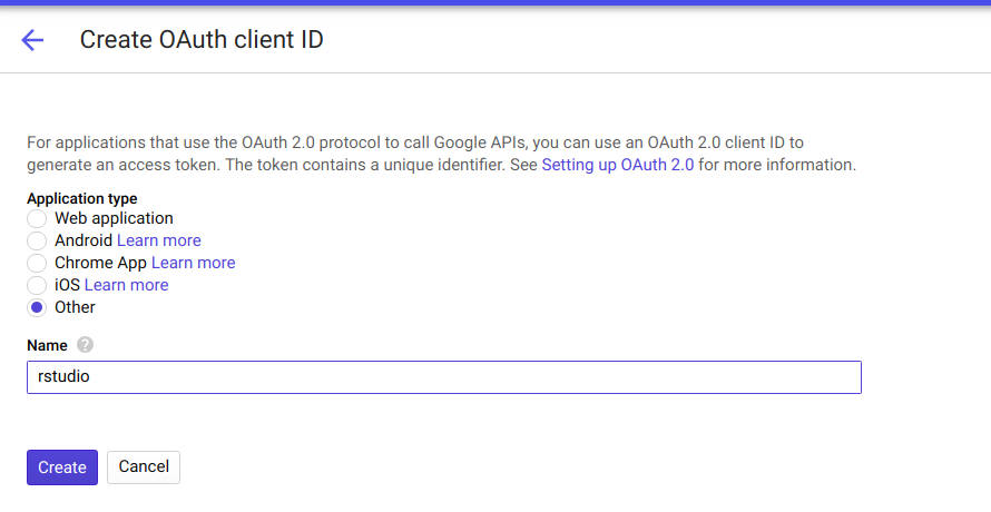
Select Other, and give your application a name. I called mine rstudio. Then click on Create.

Take note of your client ID and your client secret. These are needed in the next step!

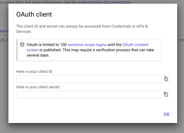
We’re done!

Using your new API credentials with gmailr

Load up gmailr and call gmail_auth() with your client ID and client secret from the previous step. These are strings, so make sure to quote them.

library(gmailr)

gmail_auth('read_only', id="your_client_id_here", secret="your_client_secret_here")

If you’re doing this for the first time, your web browser should open. You’ll be asked if you want to give your application the permission to access your Gmail account. Click on Allow if you’re keen!

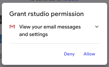
Click on Allow again.

You’ll be given another code to paste into your R console. Assuming you’re using RStudio, just go back to your console and you’ll see that the Console is waiting for some input. Paste this code there and you’re all set to go!

We’re done here, too!

Let’s get-a-searchin’

We’ll be building up to a few functions that does these things:

Download our R-bloggers emails.
Get the date and time when each email was sent.
Get the most recent blog post’s date and time.
Calculate the difference between 2 and 3, above.

Then we will get analysing!

Our targets: Identifying R-bloggers emails

I went into my gmail account and searched for emails using this string:

email_filter <- 'from:(R-bloggers <noreply+feedproxy@google.com>) subject:([r-bloggers])'

We’ll use the gmailr messages() function to get 1000 emails.

num_emails_to_get <- 1000
rbloggers_emails <- messages(search=email_filter, num_results = num_emails_to_get)

It turns out that we are using the list method of the Users.messages resource when we call the messages() function. Let’s find out more!

The response body is defined here as:

{
  "messages": [
    users.messages Resource
  ],
  "nextPageToken": string,
  "resultSizeEstimate": unsigned integer
}

The messages property is defined like this:

List of messages. Note that each message resource contains only an id and a threadId. Additional message details can > be fetched using the messages.get method.

So let’s access these message IDs so we can use the messages.get method to get more email data!

Our data is deeply-nested. Our 1,000 email IDs have been fetched in 10 chunks:

str(rbloggers_emails, 1)

## List of 10
##  $ :List of 3
##  $ :List of 3
##  $ :List of 3
##  $ :List of 3
##  $ :List of 3
##  $ :List of 3
##  $ :List of 3
##  $ :List of 3
##  $ :List of 3
##  $ :List of 3
##  - attr(*, "class")= chr "gmail_messages"

If we look at our first chunk, we can see that this structure aligns to our response body definition above!

str(rbloggers_emails[[1]], 1)

## List of 3
##  $ messages          :List of 100
##  $ nextPageToken     : chr "10088257423499543935"
##  $ resultSizeEstimate: int 103

If we focus on the messages property, we can see that each element is a pair of values.

If we look at the first pair of elements, we can can see that we have found our message id numbers!

str(rbloggers_emails[[1]][['messages']][[1]], 1)

## List of 2
##  $ id      : chr "169e04c2fd6d6450"
##  $ threadId: chr "169e04c2fd6d6450"

To get our first email id we can do this:

rbloggers_emails[[1]][['messages']][[1]][['id']]

## [1] "169e04c2fd6d6450"

Let’s wrap this up into a function and get them message IDs!

get_message_ids <- function(gmailr_obj) {
  message_ids <- character()
  for (elem in gmailr_obj) {
    messages <- elem[['messages']]
    for (i in seq_along(messages)) {
      message_ids <- append(message_ids, messages[[i]][['id']])
    }
  }
  return(message_ids)
}

message_ids <- get_message_ids(rbloggers_emails)

print(head(message_ids, 10))

##  [1] "169e04c2fd6d6450" "169db3249a0cd923" "169d616b31342c9b"
##  [4] "169d0cbeea48ac3d" "169cbd496dc9993c" "169c6d47d84bb90f"
##  [7] "169c1a4f51f2c020" "169bc32e16a346ae" "169b719ce6eb4629"
## [10] "169b1e3b25a5adf9"

Woo! Great success!

Getting more email data

We will be repeatedly calling the message function, which in turn calls the API’s Users.messages.get method of the API.

get_emails <- function(message_ids) {
  results <- list()
  for (message_id in message_ids) {
    print(sprintf('getting message id %s', message_id))
    results[[message_id]] <- message(message_id)
  }
  return(results)
}

rbloggers_emails_list <- get_emails(message_ids)

So what do we have here? Let’s look at the structure of our first resource. We’ll analyse an example_email in the next few sections:

example_email <- rbloggers_emails_list[[1]]
str(rbloggers_emails_list[[1]], 1)

## List of 8
##  $ id          : chr "169e04c2fd6d6450"
##  $ threadId    : chr "169e04c2fd6d6450"
##  $ labelIds    :List of 2
##  $ snippet     : chr "[R-bloggers] Standard Evaluation Versus Non-Standard Evaluation in R (and 9 more aRticles) Link to R-bloggers S"| __truncated__
##  $ historyId   : chr "7630366"
##  $ internalDate: chr "1554246281000"
##  $ payload     :List of 6
##  $ sizeEstimate: int 296511
##  - attr(*, "class")= chr "gmail_message"

This lines up to the resource representation found here:

{
  "id": string,
  "threadId": string,
  "labelIds": [
    string
  ],
  "snippet": string,
  "historyId": unsigned long,
  "internalDate": long,
  "payload": {
    "partId": string,
    "mimeType": string,
    "filename": string,
    "headers": [
      {
        "name": string,
        "value": string
      }
    ],
    "body": users.messages.attachments Resource,
    "parts": [
      (MessagePart)
    ]
  },
  "sizeEstimate": integer,
  "raw": bytes
}

It looks like payload contains the data we’re after - it contains the email headers, body and parts (if our message has multiple parts).

When are our emails sent?

Let’s dig into our email headers.

example_email_headers <- rbindlist(example_email$payload$headers)
example_email_sent <- example_email_headers[name=='Date', value]
print(example_email_sent)

## [1] "Tue, 02 Apr 2019 23:04:41 +0000"

The +0000 is the offset in the format +/-hhmm from UTC. Read more about it here.

This data is currently a string. Let’s convert it into a date value. To do that, we need to tell our function what each value in our date string represents. This is the final result obtained by referencing the documentation for the strptime base R function:

date_time_format <- '%a, %d %b %Y %H:%M:%S %z'

Here I have copied and pasted the relevant parts of the strptime documentation:

%a - ‘Abbreviated weekday name in the current locale on this platform. (Also matches full name on input: in some locales there are no abbreviations of names.)’
%d - ‘Day of the month as decimal number (01–31).’
%b - Abbreviated month name in the current locale on this platform. (Also matches full name on input: in some locales there are no abbreviations of names.)
%Y - ‘Year with century…’
%H - ‘Hours as decimal number (00–23).’
%M - ‘Minute as decimal number (00–59).’
%S - ‘Second as integer (00–61), allowing for up to two leap-seconds (but POSIX-compliant implementations will ignore leap seconds).’
%z - ‘Signed offset in hours and minutes from UTC, so -0800 is 8 hours behind UTC. Values up to +1400 are accepted…’

Easy! Let’s convert this into our date value using the as_datetime function from the lubridate package.

library(lubridate)

email_date_posix <- as_datetime(example_email_sent, format=date_time_format)

Where’s our email text?

There are two potential places we can look for in our the previouly mentioned Users.messages resource representation:

The payload.body attribute. Note that the documentation defines this as The message part body for this part, which may be empty for container MIME message parts..
The payload.parts[] attribute. This is defined as The child MIME message parts of this part. This only applies to container MIME message parts, for example multipart/*. For non-container MIME message part types, such as text/plain, this field is empty...

If we look at the payload.mimeType attribute, we can see that we’ve got ourselves a multipart message:

example_email$payload$mimeType

## [1] "multipart/alternative"

So by induction, the payload.body is empty…

example_email$payload$body

## $size
## [1] 0

…and payload.parts[] is not empty.

str(example_email$payload$parts,1)

## List of 2
##  $ :List of 5
##  $ :List of 5

Hooray! So let’s focus on payload.parts[].

So we have ourselves a 2 part message (a List of 2). Let’s look at the first part.

str(example_email$payload$parts[[1]],1)

## List of 5
##  $ partId  : chr "0"
##  $ mimeType: chr "text/plain"
##  $ filename: chr ""
##  $ headers :List of 2
##  $ body    :List of 2

We have some plain text (mimeType == 'text/plain') here. If we look at the headers, we can see that this text is encoded in Base64.

example_email$payload$parts[[1]]$headers[[2]]

## $name
## [1] "Content-Transfer-Encoding"
##
## $value
## [1] "base64"

Let’s look at part 2.

str(example_email$payload$parts[[2]],1)

## List of 5
##  $ partId  : chr "1"
##  $ mimeType: chr "text/html"
##  $ filename: chr ""
##  $ headers :List of 2
##  $ body    :List of 2

We have some HTML (mimeType == text/html) here. Looking at the headers for part 2, we have some quoted-printable encoded HTML.

example_email$payload$parts[[2]]$headers[[2]]

## $name
## [1] "Content-Transfer-Encoding"
##
## $value
## [1] "quoted-printable"

Either way, we can decode this to human-readable text by using gmailr's base64url_decode_to_char() function. Try these out for yourselves!

gmailr:::base64url_decode_to_char(example_email$payload$parts[[1]]$body$data)
gmailr:::base64url_decode_to_char(example_email$payload$parts[[2]]$body$data)

We will focus on part 2 - the HTML document. We will use our powers of observation to extract the posted dates.

example_email_body_html <- gmailr:::base64url_decode_to_char(example_email$payload$parts[[2]]$body$data)

We have finally found our posted dates

I originally tried to use the rvest with this XPath to locate the posted dates:

xpath = '//*[@id="itemcontentlist"]/tr/td/p[2]'

However, I was getting malformed HTML tag errors. So I resorted to using some good ol’ regex to extract the dates.

If we open up the HTML representation of our email, we can observe that the posted dates look something like this:

Posted: 29 Jan 2018 02:27 AM PST

To extract the date and time in the middle of the above string, we can use this regex pattern:

’(?<=Posted: ).+(?= )’

This regex basically says:

look for some string of 1 or more characters (.+),
that is immediately preceded by ‘Posted: ‘ ((?<=Posted: )),
and is immediately followed by ‘ ‘ ((?=))

We will use this pattern along with the stringr package’s str_extract_all() function to extract every string that matches this pattern.

library(stringr)

posted_dates <- str_extract_all(example_email_body_html, '(?<=<span>Posted:</span> ).+(?=</p>)')
posted_dates <- do.call(c, posted_dates)
print(posted_dates)

##  [1] "02 Apr 2019 09:27 AM PDT" "02 Apr 2019 05:04 AM PDT"
##  [3] "02 Apr 2019 02:59 AM PDT" "02 Apr 2019 01:00 AM PDT"
##  [5] "02 Apr 2019 12:10 AM PDT" "01 Apr 2019 06:03 PM PDT"
##  [7] "01 Apr 2019 05:23 PM PDT" "01 Apr 2019 05:00 PM PDT"
##  [9] "01 Apr 2019 05:00 PM PDT" "01 Apr 2019 05:00 PM PDT"

Success!

TIME ZONES…AAAAAAAAAARGH!!!

We can see that the posted dates have a slightly different format to the email sent date we saw earlier. Most notably:

we now have AM/PM time, and
we have a time zone abbreviation instead of a UTC offset.

The AM/PM part is easy to deal with. Dealing with time zones, however, sucks. A friend of mine (shout out to Vinay!) sent me this video from the amazing Computerphile YouTube channel. It does a great job at articulating the pain of having to deal with time zones:

R and time zones

R comes with a set of time zone names from the tz database:

tz_names <- OlsonNames()
print(tz_names)

##  [1] "Africa/Abidjan"       "Africa/Accra"         "Africa/Addis_Ababa"  
##  [4] "Africa/Algiers"       "Africa/Asmara"        "Africa/Asmera"       
##  [7] "Africa/Bamako"        "Africa/Bangui"        "Africa/Banjul"       
## [10] "Africa/Bissau"        "Africa/Blantyre"      "Africa/Brazzaville"  
## [13] "Africa/Bujumbura"     "Africa/Cairo"         "Africa/Casablanca"   
## [16] "Africa/Ceuta"         "Africa/Conakry"       "Africa/Dakar"        
## [19] "Africa/Dar_es_Salaam" "Africa/Djibouti"      "Africa/Douala"       
## [22] "Africa/El_Aaiun"      "Africa/Freetown"      "Africa/Gaborone"     
## [25] "Africa/Harare"        "Africa/Johannesburg"  "Africa/Juba"         
## [28] "Africa/Kampala"       "Africa/Khartoum"      "Africa/Kigali"       
## [31] "Africa/Kinshasa"      "Africa/Lagos"         "Africa/Libreville"   
## [34] "Africa/Lome"          "Africa/Luanda"        "Africa/Lubumbashi"   
## [37] "Africa/Lusaka"        "Africa/Malabo"        "Africa/Maputo"       
## [40] "Africa/Maseru"        "Africa/Mbabane"       "Africa/Mogadishu"    
## [43] "Africa/Monrovia"      "Africa/Nairobi"       "Africa/Ndjamena"     
## [46] "Africa/Niamey"        "Africa/Nouakchott"    "Africa/Ouagadougou"  
## [49] "Africa/Porto-Novo"    "Africa/Sao_Tome"     
##  [ reached getOption("max.print") -- omitted 557 entries ]

What are the time zone abbreviations in the R-bloggers posted dates?

Let’s use some regex!

posted_date_tz_pat <- '(?<=[0-9]{2}:[0-9]{2} (AM|PM) )\\w+$'
posted_date_tz <- sapply(posted_dates, function(x) str_extract(x, posted_date_tz_pat))

PDT doesn’t exist in R’s OlsonNames. Doing some research, we can see that PDT refers to Pacific Daylight Time, which is the daylight saving time of the Pacific Time Zone. The non-daylight saving time (i.e. standard time) variant is Pacific Standard Time, which has an abbreviation of PST. The UTC offsets for PST and PDT are:

PST == -08:00, and
PDT == -07:00

If we look at this Wikipedia article, we have a table named List. We observe that there are two columns that map to standard time and daylight saving time:

UTC offset +/hh:mm
UTC DST offset +/hh:mm

If we scroll through our list, we can see that there are several time zones that match our PST and PDT offsets. One of those is America/Los_Angeles. Does this exist in the time zone database?

'America/Los_Angeles' %in% tz_names

## [1] TRUE

Yes, it does! So let’s use it.

We now have all the parts we need to write some functions that go through all of our emails and extract the date the email was sent and the latest posting date. We can use this information to figure out when we should be posting our articles!

Putting it all together

We’ll write something like this:

results = empty data table

for each email:
  # deal with email date
  email_date = get_email_date(email)
  email_date_value = convert_date_to_date_value(email_date)

  # deal with posted dates
  posted_dates = get_posted_dates(email)
  posted_date_values = convert_posted_dates_to_date_values(posted_dates)
  latest_posted_date = max(posted_date_values)

  # create our row to append to results table
  row_to_append = [email_date, date_value, latest_posted_date]

  # append!
  results = append(results, row_to_append)

# once we have gone through all our emails, create some date features like
# hour email sent, minute email sent etc.
results = create_date_features(results)

Getting the email date

This is what we’ll do:

Pass in one of our emails in our email list to our function
Get the email’s header information. Create a data.table that contains a name field and a corresponding value field.
Subset this data.table and return the string representing the date and time the email was sent.

get_email_date <- function(email_obj) {
  headers <- as.data.table(do.call(rbind, email_obj$payload$headers))
  email_date <- headers[name=='Date', value][[1]]
  return(email_date)
}

NEXT!

Getting our ‘Posted’ dates

We’ll wrap our Base64 decoding logic and regex in a function that returns a vector of ‘posted dates’.

get_posted_dates <- function(email_obj) {
  email_body_base64 <- email_obj$payload$parts[[2]]$body$data
  email_body_html <- gmailr:::base64url_decode_to_char(email_body_base64)
  posted_dates <- str_extract_all(email_body_html, '(?<=<span>Posted:</span> ).*(?=</p>)')
  posted_dates <- do.call(c, posted_dates)
  return(posted_dates)
}

Converting our email header ‘Date’ into date time values

We know what our email date format is from before. So we will do this:

Pass in the date and time string from the previous function.
Convert this into a POSIXlt type using as_datetime.
Coerce the POSIXlt object into a POSIXct object.

The practical consequence of using POSIXct instead of POSIXlt is that with POSIXct, we get a single date-time object that can be displayed as you would expect in a field in a table. POSIXlt, on the other hand, returns a named vector that allows you to split the date-time object into its component parts. For example:

example_datetime <- as.POSIXlt('2019-01-01 10:11:23', tz='UTC')
class(example_datetime)

## [1] "POSIXlt" "POSIXt"

We can now unlist this POSIXlt object to see what it’s made up of:

unlist(example_datetime)

##   sec   min  hour  mday   mon  year  wday  yday isdst
##    23    11    10     1     0   119     2     0     0

When we use POSIXlt types in data.frames or anything that inherits from a data.frame, some implicit coercion is done that turns it into a POSIXct type:

example_df <- as.data.frame(example_datetime)
class(example_df$example_datetime)

## [1] "POSIXct" "POSIXt"

But we will take care of this in our function just to be sure. Here’s the final product:

convert_email_date <- function(email_date_str) {
  email_date_posix <- as_datetime(email_date_str, format='%a, %d %b %Y %H:%M:%S %z')
  return(as.POSIXct(email_date_posix))
}

Convert our ‘Posted’ dates into date values

This follows a slightly different pattern.

We know that our time zone of interest is America/Los_Angeles from our above analysis. We will therefore do this:

Extract the date and time portion of our posted dates and discard our PDT and PST time zone abbreviations.
Convert our dates and times into POSIXlt types, specifying the America/Los_Angeles time zone.
Offset our POSIXlt date times to the UTC time zone using lubridate's with_tz() function.
Convert our values into POSIXct objects. We will be using lapply instead of sapply here because sapply coerces our dates into integers instead of retaining our desired POSIXct type.
Return our vector of UTC date times.

We can then take the max() of this vector in our main function (which we will be writing below).

convert_posted_dates <- function(posted_dates) {
  # get the date and time only as we know what the tz is from our above analysis
  without_tz_pat <- '(\\d{2} \\w{3} \\d{4} \\d{2}:\\d{2} (?:AM|PM))'
  date_time_only <- str_extract_all(posted_dates, without_tz_pat)
  date_time_only <- do.call(c, date_time_only)

  # convert the date time into a date time value using the posted date time zone
  date_time_format <- '%d %b %Y %I:%M %p'
  date_time_values <- as_datetime(date_time_only, format=date_time_format,  tz='America/Los_Angeles')

  # convert to UTC time
  date_time_values_utc <- with_tz(date_time_values, tzone='UTC')

  # convert to POSIXct
  date_time_values_utc <- lapply(date_time_values_utc, as.POSIXct)
  date_time_values_utc <- do.call(c, date_time_values_utc)

  return(date_time_values_utc)
}

Creating email date and time ‘features’

We might not use a lot of these in our analysis, but let’s create more than we need just in case we want to analyse them later.

create_date_features <- function(email_date_dt) {
  email_date_dt[, `:=`(
  email_date = date(email_date_posix),
  email_day = day(email_date_posix),
  email_month = month(email_date_posix),
  email_year = year(email_date_posix),
  email_weekday = wday(email_date_posix),
  email_hour = hour(email_date_posix),
  email_minute = minute(email_date_posix),
  email_second = second(email_date_posix),
  diff_mins_max_post_to_email_date = difftime(latest_posted_date, email_date_posix, unit='mins')
  )]
  return(email_date_dt)
}

Our main function

Time to put it all together!

make_email_dates_dt <- function(emails_list) {

  result <- data.table()

  for (email in emails_list) {
    email_id <- email$id

    # deal with our email header `Date`
    email_date <- get_email_date(email)
    email_date_posix <- convert_email_date(email_date)

    # deal with our posted dates
    posted_dates <- get_posted_dates(email)
    posted_dates_posix <- convert_posted_dates(posted_dates)
    max_posted_date <- max(posted_dates_posix)

    # create our intermediate results
    temp_result <- data.table(email_id=email_id, email_date=email_date,
                              email_date_posix=email_date_posix,
                              latest_posted_date = max_posted_date)

    result <- rbind(result, temp_result)
  }

  result <- create_date_features(result)

  return(result)
}

And execute it!

email_dates <- make_email_dates_dt(rbloggers_emails_list)
head(email_dates[, 1:4], 5)

Sweet as. We good.

Analysis time

How many emails per day?

Sometimes, more than one email is sent per day when we use the UTC ‘Date’ in the email headers. For example, if you search for these emails using the Gmail search box, you will see that they both were sent on 29 Mar 2019:

[R-bloggers] Using RStudio and LaTeX (and 6 more aRticles) [R-bloggers] Securing a dockerized plumber API with SSL and Basic Authentication (and 3 more aRticles)

One was sent just after 12 AM on 29-Mar-2019, and the other was sent just before 12 AM on 30-Mar-2019.

What happens when we look at these date times in Pacific Time?

ymd_hm('2019-03-29 00:00') %>%
  with_tz(tzone='America/Los_Angeles') %>%
  print()

## [1] "2019-03-28 17:00:00 PDT"

ymd_hm('2019-03-30 00:00') %>%
  with_tz(tzone='America/Los_Angeles') %>%
  print()

## [1] "2019-03-29 17:00:00 PDT"

They fall on different dates! Let’s keep this in mind for later when we backtest our strategy because it will be important.

In which hour are these emails sent?

Let’s see what we have:

count_per_hour <- email_dates[, .N, email_hour][order(email_hour), ]
print(count_per_hour)

##    email_hour   N
## 1:          0 249
## 2:          1  13
## 3:          2   3
## 4:         22 244
## 5:         23 491

It looks like emails aren’t sent randomly across the 24 hours of the day. This is a good sign. To plot these nicely, we will fill our data.table with the missing hours of the day to get a full set of 24 hours.

missing_hours <- setdiff(0:23, count_per_hour$email_hour)
missing_hours <- data.table(email_hour=missing_hours, N=rep(0, length(missing_hours)))
count_per_hour <- rbind(count_per_hour, missing_hours)

ggplot(count_per_hour, aes(email_hour, N)) +
  geom_point(alpha=0.7) +
  labs(title='Hour email sent according to header') +
  scale_x_continuous(breaks = 0:23) +
  labs(x = 'Hour of day')

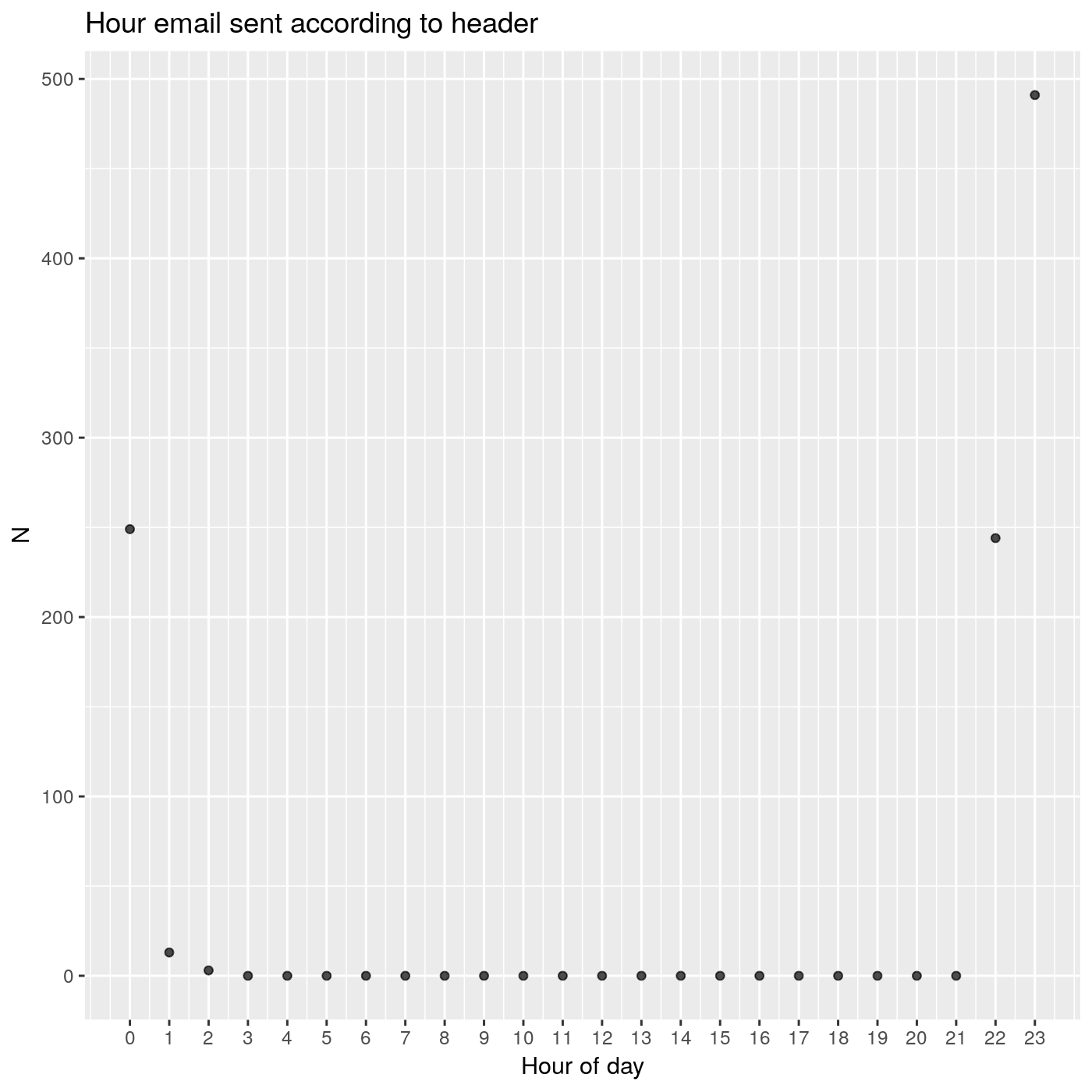
We have the majority of emails being sent between 22:00 UTC and 00:00 UTC.

How has the email-hour varied across time?

This was interesting!

ggplot(email_dates, aes(email_month, email_hour)) +
  geom_jitter(alpha=0.2) +
  labs(title='Hour email sent by year') +
  scale_y_continuous(breaks=0:23) +
  scale_x_continuous(breaks=1:12) +
  facet_wrap(~email_year) +
  labs(x = 'Month of year', y = 'Hour of day')

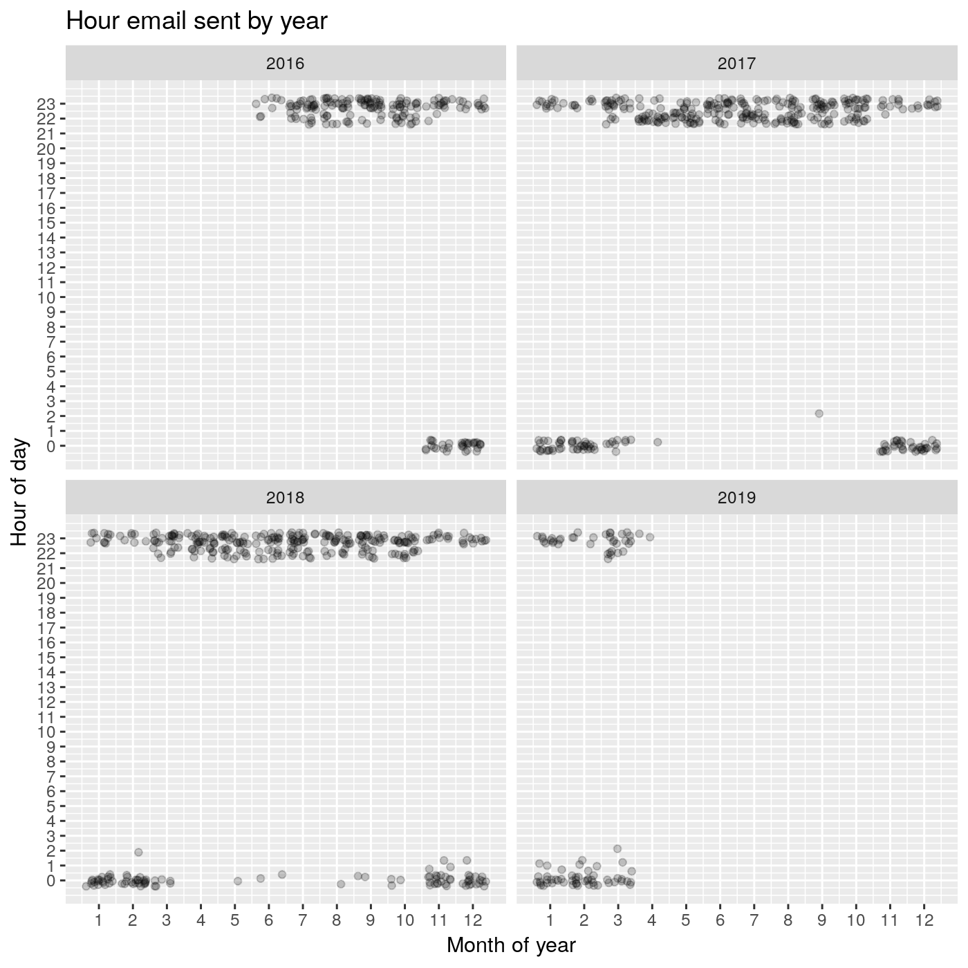
What do we have here? It looks like between the end of the year and the beginning of the next year, emails are more likely to be sent at about 00:00 UTC. They are more likely to be sent about 23:00 UTC in the rest of the year. The Posted dates in the R-bloggers emails themselves reveals why this may be the case.

Remember that we converted the PDT and PST Posted dates into UTC? According to this Wikipedia article:

Effective in the U.S. in 2007 as a result of the Energy Policy Act of 2005, the local time changes from PST to PDT at 02:00 LST to 03:00 LDT on the second Sunday in March and the time returns at 02:00 LDT to 01:00 LST on the first Sunday in November.

What does this mean for us? It means that depending on the date, we should be sending our emails at different times of the day depending on which month of the year we are in!

Conclusion: our anchor hours

Let’s make a call and use these hours as anchor points to define how far before these anchor points we should be posting to make it to the top of the list! Just to be safe, we will be using the earliest likely hour an email is sent. We base this on observing the above plot! So, we will be using:

hour 22 in the months from March through to October, inclusive

and

hour 23 in the months from November to Februrary, inclusive.

What about the minute in which the emails are sent?

Let’s try to figure out which minute of the hour we should be aiming to post before depending on what month of the year we are in.

counts_minutes_per_hour <- email_dates[, .N, .(email_month, email_hour, email_minute)]

ggplot(counts_minutes_per_hour, aes(email_minute, N)) +
  geom_histogram(stat='identity') +
  labs(title='Minute email sent by hour of day and month of year', subtitle="", x='Minute of hour') +
  facet_grid(email_month~email_hour)

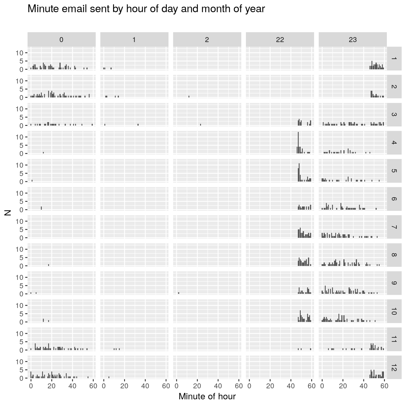
We have the hour of day represented in columns and we have the month of year represented in rows. Within each subplot, we have minute within the hour. Based on this big plot, regardless of which month of the year we are in, sending before the 40th minute looks like a good idea.

Conclusion - our final anchor times:

Let’s make another call! Our final anchor points are:

22:40 in the months from March through to October, inclusive

and

23:40 in the months from November to Februrary, inclusive.

What is our window of opportunity?

Here, we want to figure out how many minutes prior to the email header 'Date' the most recent post was made. If we set our post date time to a value too close to the posted date time, we run the risk of missing that day’s email and ending up at the very bottom of the next day's email! So let’s keep this in mind as we continue our analysis.

Let’s arbitrarily say that we are happy with being at the top of the list 90% of the time. Let’s find out what this 90% cut-off corresponds to in minutes:

quantile(email_dates$diff_mins_max_post_to_email_date, seq(0, 1, 0.05))

## Time differences in mins
##           0%           5%          10%          15%          20%
## -9277.916667 -1441.787500 -1015.878333  -787.493333  -671.523333
##          25%          30%          35%          40%          45%
##  -597.975000  -534.486667  -481.711667  -456.500000  -434.389167
##          50%          55%          60%          65%          70%
##  -415.383333  -392.657500  -369.176667  -338.105000  -298.441667
##          75%          80%          85%          90%          95%
##  -255.262500  -223.033333  -193.909167  -150.510000   -81.077500
##         100%
##    -2.733333

The answer is about 150 minutes.

Conclusion - our target posting date time

Let’s do it! We will go with a value of 150 minutes (i.e 2.5 hours) before our previously defined anchor points. This corresponds to:

20:10 UTC in the months from March through to October, inclusive

and

21:10 UTC in the months from November to Februrary, inclusive.

Time to get backtesting!

To backtest our strategy, we might initially think of taking our UTC email 'Date' from our header, applying our target posting time from the immediately preceding section, and see whether I have beaten the latest post on that day. Let’s try something like this:

email_dates[ , target_date := if_else(
  email_month %in% 3:10,
  ymd_hm(paste(email_date, '20:10', tz='UTC')),
  ymd_hm(paste(email_date, '21:10', tz='UTC'))
)]

email_dates[, `:=`(
  target_after_latest = target_date > latest_posted_date,
  target_before_email = target_date < email_date_posix
)]

email_dates[ , i_win := target_after_latest & target_before_email]

We see that our performance is not as good as we would have liked!

email_dates[, .N, i_win]

##    i_win   N
## 1:  TRUE 646
## 2: FALSE 354

Hmmmmm…what is happening here?

Revisiting multiple posts on the same day

In the above How many emails per day? section, we discovered that when we convert our UTC date times into PT date times, what looked like multiple posts per day turned out to be posts on different days.

To deal with this dynamic, let’s create a PT date time column, add our posting hours and coerce the resulting date time to the UTC time zone.

email_dates[ , email_date_pt := date(with_tz(email_date_posix, tzone='America/Los_Angeles'))]

email_dates[ , target_date := if_else(
  email_month %in% 3:10,
  ymd_hm(paste(email_date_pt, '20:10', tz='UTC')),
  ymd_hm(paste(email_date_pt, '21:10', tz='UTC'))
)]

email_dates[, `:=`(
  target_after_latest = target_date > latest_posted_date,
  target_before_email = target_date < email_date_posix
)]

email_dates[ , i_win := target_after_latest & target_before_email]

Let’s look at our performance now:

email_dates[, .N, i_win]

##    i_win   N
## 1:  TRUE 859
## 2: FALSE 141

Hooray! ~86% is close enough to 90% for me. But lets have some fun and keep going!

Let’s push it to the limit!

How many more wins can we gain if we pushed our target dates closer to the email sent dates?

Let’s say we want to sweep across a range of minutes to add to our original target posting dates and times.

max_minutes_to_add <- 60*3

We’ll use a good-ol’ for loop and iteratively build out a data.table containing our results.

wins <- data.table()

for (i in seq(0, max_minutes_to_add)) {
  my_email_dates <- email_dates$target_date + minutes(i)
  i_win <- sum(my_email_dates > email_dates$latest_posted_date & my_email_dates < email_dates$email_date_posix)
  temp_results <- data.table(mins_before_anchor = i, wins = i_win, win_pct = i_win/nrow(email_dates))
  wins <- rbind(wins, temp_results)
}

Let’s take a look at our results:

ggplot(wins, aes(x=mins_before_anchor, y=win_pct)) +
  geom_point(stat='identity', alpha=0.5) +
  scale_y_continuous(labels = scales::percent) +
  labs(title='How many more wins could we get?',
       subtitle='Push it to the limit...(LIMIIIIIIIT!)',
       x='Minutes after our target posting dates and times',
       y='Percentage of wins')

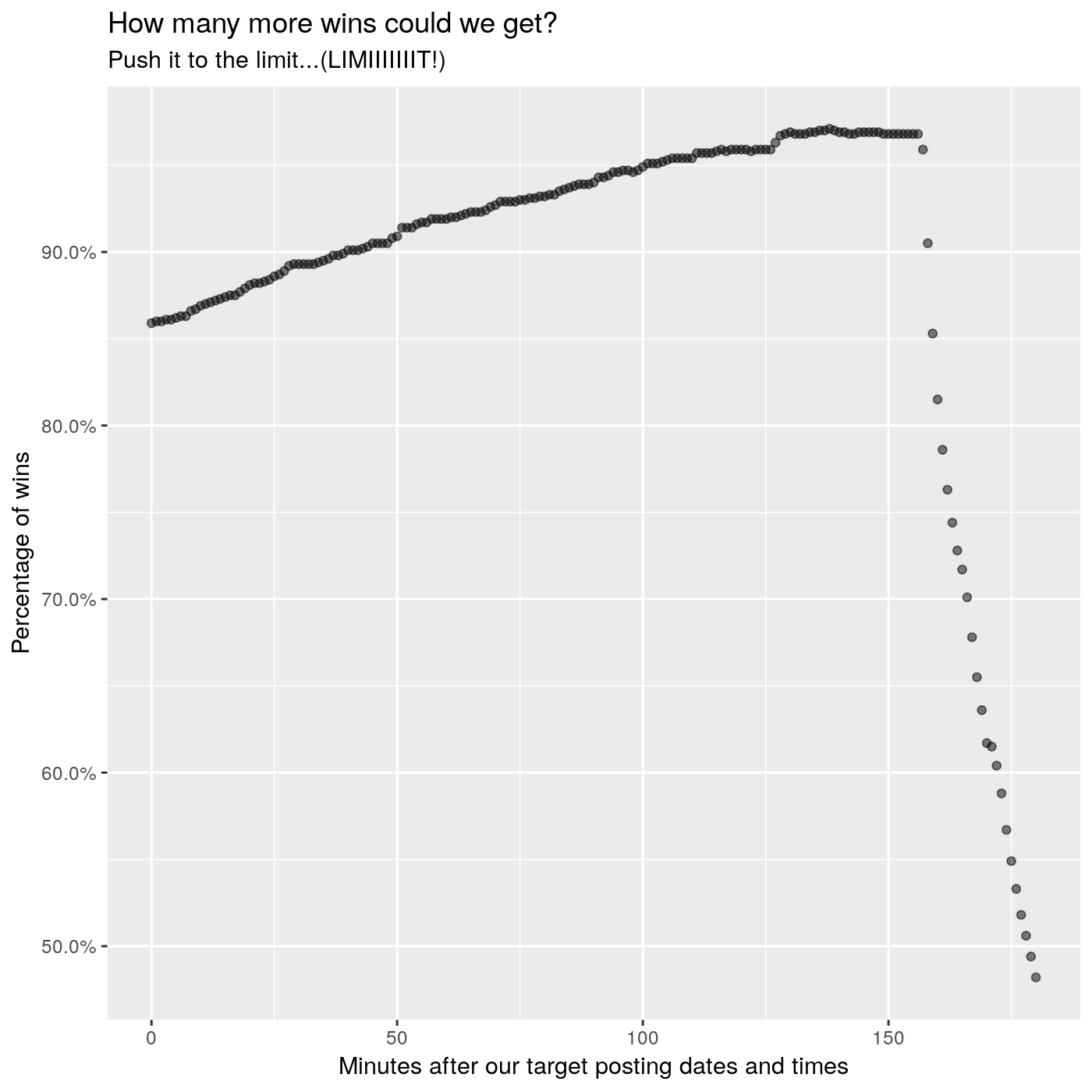
Yes, we can definitely push our posting times further into the future. But if we push them too much, we end up becoming the first post of the next email. The first post is listed last, so we end up right at the bottom!

Let’s arbitrarily go with 100 additional minutes on top of our original target dates and times…because 100 is a nice number! Our strategy then becomes this:

21:50 UTC in the months from March through to October, inclusive

and

22:50 UTC in the months from November to Februrary, inclusive.

email_dates[ , target_date := if_else(
  email_month %in% 3:10,
  ymd_hm(paste(email_date_pt, '21:50', tz='UTC')),
  ymd_hm(paste(email_date_pt, '22:50', tz='UTC'))
)]

email_dates[, `:=`(
  target_after_latest = target_date > latest_posted_date,
  target_before_email = target_date < email_date_posix
)]

email_dates[ , i_win := target_after_latest & target_before_email]

And our performance?

email_dates[, .N, i_win]

##    i_win   N
## 1:  TRUE 949
## 2: FALSE  51

About 95%!

Conclusion

Let’s write a simple function that simply tells us when to post:

when_should_i_post <- function() {
  todays_date_utc <- with_tz(Sys.time(), tzone='UTC')

  if (month(todays_date_utc) %in% 3:10) {
    hour(todays_date_utc) <- 21
    minute(todays_date_utc) <- 50
  } else {
    hour(todays_date_utc) <- 22
    minute(todays_date_utc) <- 50
  }
  second(todays_date_utc) <- 0
  post_at <- with_tz(todays_date_utc, tzone='Australia/Sydney')
  return(post_at)
}

And our answer:

when_should_i_post()

## [1] "2019-04-04 08:50:00 AEDT"

Unfortunately, I have a job so I guess I won’t be able to post then anyway!

Justin.

Share on

Twitter Facebook LinkedIn

Hello, world!
My name is Justin.

(Trying) to get to the top of R-bloggers emails

Where the data at? - gmailr

Some prework - enabling the Gmail API

Using your new API credentials with gmailr

Let’s get-a-searchin’

Our targets: Identifying R-bloggers emails

Getting more email data

When are our emails sent?

Where’s our email text?

We have finally found our posted dates

TIME ZONES…AAAAAAAAAARGH!!!

R and time zones

What are the time zone abbreviations in the R-bloggers posted dates?

Putting it all together

Getting the email date

Getting our ‘Posted’ dates

Converting our email header ‘Date’ into date time values

Convert our ‘Posted’ dates into date values

Creating email date and time ‘features’

Our main function

Analysis time

How many emails per day?

In which hour are these emails sent?

How has the email-hour varied across time?

Conclusion: our anchor hours

What about the minute in which the emails are sent?

Conclusion - our final anchor times:

What is our window of opportunity?

Conclusion - our target posting date time

Time to get backtesting!

Revisiting multiple posts on the same day

Let’s push it to the limit!

Conclusion

Share on

You may also enjoy

Statistical significance intuition

Faster web scraping with Python and asyncio

How to plan your life

An antidote to hustle culture: a better way to manage your time

Hello, world! My name is Justin.

Where the data at? - gmailr

Some prework - enabling the Gmail API

Using your new API credentials with gmailr

Let’s get-a-searchin’

Our targets: Identifying R-bloggers emails

Getting more email data

When are our emails sent?

Where’s our email text?

We have finally found our posted dates

TIME ZONES…AAAAAAAAAARGH!!!

R and time zones

What are the time zone abbreviations in the R-bloggers posted dates?

Putting it all together

Getting the email date

Getting our ‘Posted’ dates

Converting our email header ‘Date’ into date time values

Convert our ‘Posted’ dates into date values

Creating email date and time ‘features’

Our main function

Analysis time

How many emails per day?

In which hour are these emails sent?

How has the email-hour varied across time?

Conclusion: our anchor hours

What about the minute in which the emails are sent?

Conclusion - our final anchor times:

What is our window of opportunity?

Conclusion - our target posting date time

Time to get backtesting!

Revisiting multiple posts on the same day

Let’s push it to the limit!

Conclusion

Share on

You may also enjoy

Statistical significance intuition

Faster web scraping with Python and asyncio

How to plan your life

An antidote to hustle culture: a better way to manage your time

Hello, world!
My name is Justin.