I walk the (train) line - part deux - the weight loss continues
(TL;DR: author continues to use his undiagnosed OCD for good. Breath-first search introduced on simple graph.)
We learnt how to get OpenStreetMap data into R last time. And I said that we will be doing a little bit of this:
So what the hell is this?
This is an example of breadth-first search of a graph. We will be using it to answer this question:
Does a path exists between our source node and our destination node?
A little bit of background
To understand breadth-first search, we first need to understand:
- the concept of adjacent nodes in graphs,
- the adjacency list representation of a graph,
- the queue data structure.
I will systematically attack these as usual.
What does adjacent mean?
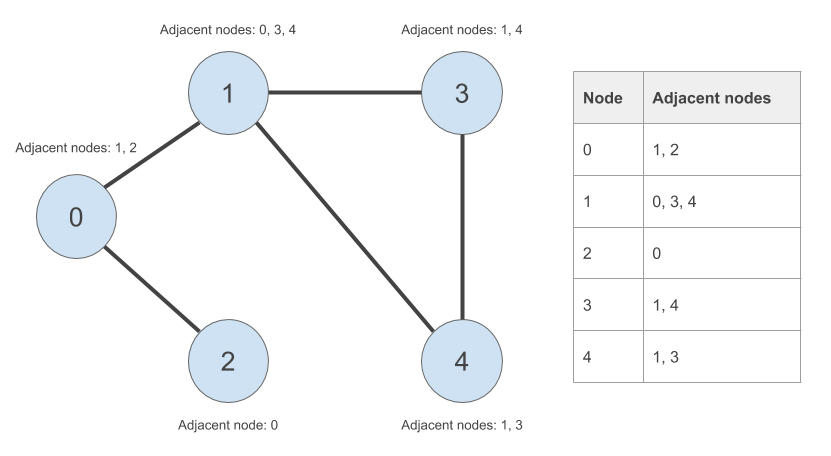
Here is our undirected graph from part one of this multi-part epic with one change - I have given the nodes ID numbers from 0 to 4, inclusive:
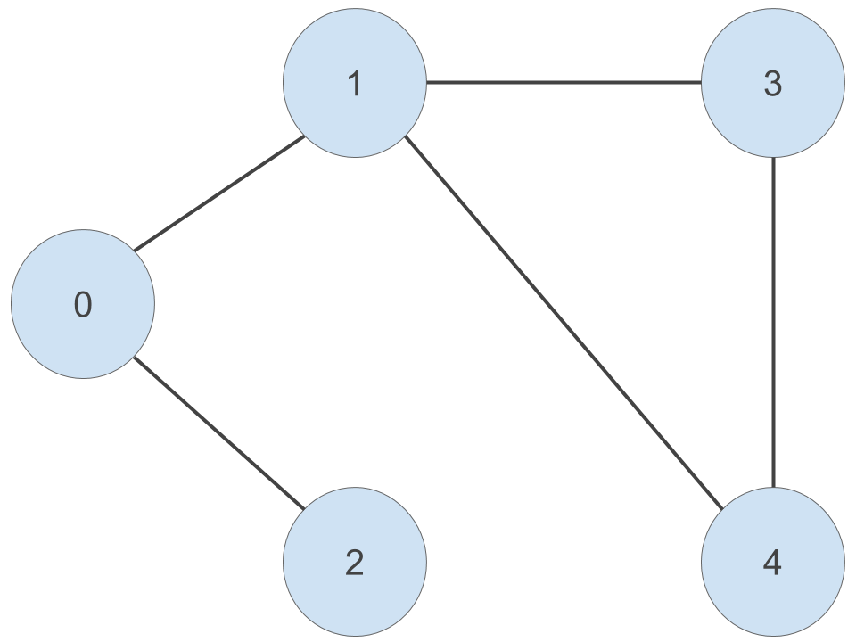
Given a particular node, a node that is adjacent to this node is another node that is connected to it by an edge. For example, node ‘0’ is connected to node ‘1’ and node ‘2’ by an edge. So we can say that node ‘1’ and node ‘2’ are adjacent to node ‘0’. Because this is an undirected graph, this relationship is symmetric - node ‘0’ is adjacent to node ‘1’ and node ‘2’.
We can apply this concept to our graph of roads. Here, we arbitrarily pick a starting node (the green one), and progressively highlight the next adjacent nodes in the direction away from the starting node. Each node is coloured differently by the smallest number of edges it takes to reach it from our starting node:
- Red = 1 edge
- Blue = 2 edges
- Orange = 3 edges
- Purple = 4 edges
- Pink = 5 edges
‘Define adjacent’ - check.
What is an adjacency list represenation of a graph?
An adjacency list is a data structure that can be used to answer this question:
Given all the nodes in our graph, which nodes are they adjacent to?
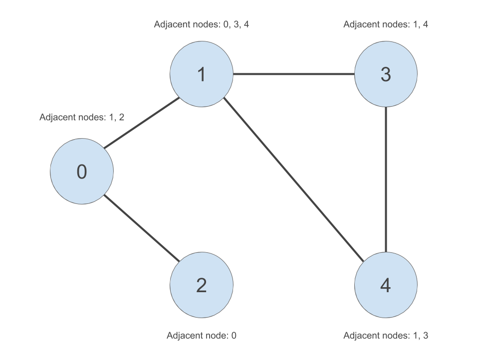
We will simply create a list of vectors data structure in R. We will firstly create a list of unique node IDs. Then for each node ID in our list, we will create a vector of nodes adjacent to those node IDs. The adjacency list is shown in the table to the right in the below image:
‘Define adjaceny lists’ - check.
Queues!
This one is slightly more complex. The analogy that is often used is that of a bus stop. Here is that analogy, illustrated with an icon from the Noun Project and some old, old memes.
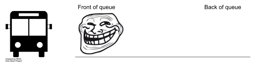
This, ladies and gentlemen, is a bus stop:

In order to get trolling first thing in the morning, Trollface shows up first. He joins the queue (i.e. is enqueued):
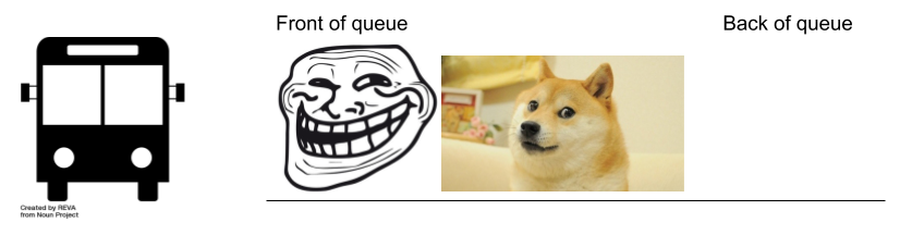
Good girl wants to go for an early walk, so Doge shows up second. She joins the queue from the back (i.e. is enqueued from the back):
Nicolas Cage meme shows up late to the party, so he joins the queue in last place (i.e. is enqueued from the back):

In what order are they going to get onto the bus? Assuming that everyone respects the unwritten rules of the queue, Trollface will leave the queue first (i.e. is dequeued first). Then Doge. Then Nic:

How is this relevant to graphs?
My claim is that, if we replace these old memes with graph nodes, the queue data structure and our adjacency list can be used to perform a breath-first search of our graph. This breadth-first search will show us whether a path exists from our source node to our destination node. We will finally get to this later on in this post (I promise!).
But first, let’s work on this ridiculous queue example to see how we can use queues in R.
rstackdeque
We will be using the lightning fast rstackdeque package instead of creating our queue data structure from scratch. The elements of the queue are individual environments, containing some data and a reference to the next environment (see here for more juicy details).
library(rstackdeque)
Let’s create an empty queue:
bus_stop_q <- rpqueue()
print(bus_stop_q)
## A queue with 0 elements.
Let’s insert Trollface and Doge:
bus_stop_q <- insert_back(bus_stop_q, 'trollface')
bus_stop_q <- insert_back(bus_stop_q, 'doge')
print(bus_stop_q)
## A queue with  2  elements.
## Front:
##  $: chr "trollface"
##  $: chr "doge"
‘trollface’ is at the front, and ‘doge’ is at the back of our queue. Success!
Inserting Nicolas Cage meme, we get:
bus_stop_q <- insert_back(bus_stop_q, 'nicolas_cage')
print(bus_stop_q)
## A queue with  3  elements.
## Front:
##  $: chr "trollface"
##  $: chr "doge"
##  $: chr "nicolas_cage"
Hooray!
Now for dequeueing. When we dequeue, we want to keep track of two things:
- the element that was deqeued from the front (i.e. which meme was dequeued from the front?), and
- the queue with the front-most element removed (i.e. the state of the bus stop after dequeueing)
We have to do this in two steps. Firstly, keeping track of the dequeued element:
dequeued <- peek_front(bus_stop_q)
print(dequeued)
## [1] "trollface"
Then, the queue without the dequeued element:
bus_stop_q <- without_front(bus_stop_q)
print(bus_stop_q)
## A queue with  2  elements.
## Front:
##  $: chr "doge"
##  $: chr "nicolas_cage"
Easy! We can keep dequeueing until the queue is empty. We can use the empty() function to define this terminating condition.
empty(bus_stop_q)
## [1] FALSE
Let’s process the remaining elements of the queue until it’s empty:
while (!empty(bus_stop_q)) {
  dequeued <- peek_front(bus_stop_q)
  print(dequeued)
  bus_stop_q <- without_front(bus_stop_q)
}
## [1] "doge"
## [1] "nicolas_cage"
Done!
Adjacency lists in R
Instead of using a package, let’s write these from scratch. Let’s use our undirected graph to take us away from our old memes and into the wonderful world of graphs. Here is our graph again:
Let’s create our outer list. We should have an element for every node in our graph.
Note: In hindsight, I shouldn’t have zero-indexed the node numbers! But I am in too deep so will have to work around my mistake.
adjacency_list <- rep(list(NULL), 5)
names(adjacency_list) <- c('0', '1', '2', '3', '4')
For every node, we will painstakingly create a vector containing the nodes adjacent to the respective node:
adjacency_list[['0']] <- c('1', '2')
adjacency_list[['1']] <- c('0', '3', '4')
adjacency_list[['2']] <- '0'
adjacency_list[['3']] <- c('1', '4')
adjacency_list[['4']] <- c('1', '3')
Here is our adjacency list:
print(adjacency_list)
## $`0`
## [1] "1" "2"
##
## $`1`
## [1] "0" "3" "4"
##
## $`2`
## [1] "0"
##
## $`3`
## [1] "1" "4"
##
## $`4`
## [1] "1" "3"
You are now ready for the breath-first search algorithm.
Breadth-first search…finally!
So what is this breadth-first search?
When performing breadth-first search, we start with a source node. We visit every child of the source node. Then for every child of the source node, we visit every one of their children. We continue this process of visiting nodes at the same level of the graph until some condition is met (for example, we have reached our destination node). That’s why it looks like nodes are being visited in concentric circles about the green node (i.e. source node), moving broader before moving deper into the graph in the initial gif:
Let’s apply this to our undirected graph. Our breadth-first search toolbox contains these things:
- our adjacency list representation of our graph,
- a source node,
- a destination node,
- our queue data structure, and
- a vector keeping track of which nodes we have already visited and from which nodes we came from when we visited them (bare with me here)
What is this vector of visited nodes?
The vector in the last point is used to avoid going in cycles as we visit nodes in our graph. For example, we start at node ‘0’. Node ‘0’ is adjacent to node ‘1’. Later on in our breadth-first search, there will come a time when we need to process the nodes adjacent to node ‘1’. When this happens, we want to avoid processing node ‘0’ again as we have already visited it. Otherwise, we will enter an infinite loop whereby we visit node ‘0’, which is adjacent to node ‘1’, which is adjacent to node ‘0’ and so on.
A little detail relevant to creating this vector of visited nodes - what is the predecessor of the source node?
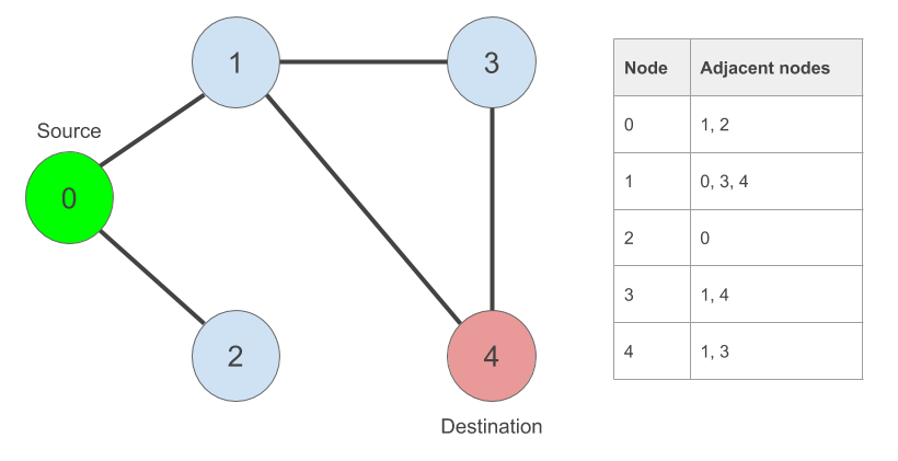
In our graph, our source node is ‘0’. Our destination node is ‘4’. We can clearly see that there is a way to get from ‘0’ to ‘4’. But it won’t be this obvious in a larger graph.
Let’s create them:
source_node <- '0'
destination_node <- '4'
Here is our vector of visited nodes. We will be keeping track of the nodes we came from when we visit each one of them.
visited_nodes <- rep(NA_character_, length(adjacency_list))
names(visited_nodes) <- names(adjacency_list)
Our source node has no predecessor! So we will simply set its predecessor to itself:
visited_nodes[source_node] <- source_node
print(visited_nodes)
##   0   1   2   3   4
## "0"  NA  NA  NA  NA
Done.
Finally, finally, finally! The breadth-first search algorithm in pseudo code
Here it is:
# create flag to indicate whether we have found our destination node
found = FALSE

create new queue
enqueue source node

while found == FALSE or the queue has elements left to process:
  dequeue node at front of queue
  if dequeued node == destination node:
    found = TRUE
  else:
    for every child of the dequeued node:
      if it has not been visited yet:
        enqueue child node at back of queue
        mark child node as visited from dequeued node
      end if
    end for
  end if
end while
The neat thing about this algorithm is that, if we find our destination node, we can recover the path the algorithm took to reach it from the source node. Let’s assume that we found our destination node ‘4’ and that our ‘visited_nodes’ vector looks like this:
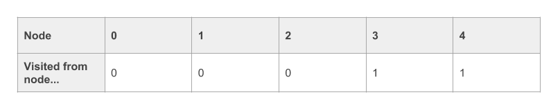
To recover the path, we can do something like this. We start with the destination node, and work backwards:
current_node = destination_node
path = current_node

while visited_nodes[current_node] != source_node:
    current_node = visited_nodes[current_node]    # find predecessor of current_node
    path = append(path, current_node)             # append it to our path
end while

# once we have reached our source_node, we simply append it to our path
path = append(path, source_node)

# we have found our path in reverse order (from destination to source). we
# reverse it to find a path from source to destination
path = reverse(path)
The breadth-first search algorithm in R
Let’s write a breath-first search function…but first, a little sidenote.
Sidenote: learning algorithms
Algorithms can be difficult to digest. I would recommend writing a function containing the algorithm and then using the handy debug() function to step through it. All you have to do is this:
debug(<function_name>)
Then call the function as you would normally:
<function_name>(<function_args>)
And then, if you’re using RStudio, you can step through it line-by-line using the F10 key. You can print the values of the local variables of your function using the R console to see how they evolve.
Once you’re done with debugging, you need to tell R to stop debugging the function. This is done like this:
undebug(<function_name>)
Enough! Here is the algorithm
bfs <- function(adjacency_list, source_node, destination_node) {
  require(rstackdeque)

  # some initial checks
  if (!source_node %in% names(adjacency_list)) {
    print('source node not in this graph...')
    return()
  }

  if (!destination_node %in% names(adjacency_list)) {
    print('destination node not in this graph...')
    return()
  }

  # initialise our 'found destination node' flag
  found <- FALSE

  # set up our visited nodes vector
  visited_nodes <- rep(NA_character_, length(adjacency_list))
  names(visited_nodes) <- names(adjacency_list)

  # initialise source node predecessor as itself
  visited_nodes[source_node] <- source_node

  # create our empty queue and enqueue source node
  q <- rpqueue()
  q <- insert_back(q, source_node)

  while(!found | !empty(q)) {
    # dequeue at front element
    dequeued_node <- peek_front(q)
    q <- without_front(q)
    # have we found our destination node?
    if (dequeued_node == destination_node) {
      found <- TRUE
    } else {
      # otherwise, we have nodes to process. process each child
      # of the dequeued node...
      for (child_node in adjacency_list[[dequeued_node]]) {
        # ...only if we have not visited it yet
        if(is.na(visited_nodes[child_node])) {
          # enqueue child node
          q <- insert_back(q, child_node)
          # mark the child node as visited from the dequeued node
          visited_nodes[child_node] <- dequeued_node
        }
      }
    }
  }

  # if we still have not found our path, it does not exist
  if (!found) {
    print('path not found')
    return()
  }

  # otherwise, recover the path from destination to source
  path <- character()
  current_node <- destination_node
  path <- append(path, current_node)

  while (visited_nodes[[current_node]] != source_node) {
    current_node <- visited_nodes[[current_node]]
    path <- append(path, current_node)
  }
  path <- append(path, source_node)

  # and then reverse it!
  path <- rev(path)

  return(path)
}
Let’s test it out:
bfs(adjacency_list, source_node, destination_node)
## [1] "0" "1" "4"
Good…good..
As suspected, there is a path from our source node to our destination node. The path that the algorithm found in this case was 0 -> 1 -> 4.
My crappy animation
Here is my terrible attempt at animating the algorithm. Hopefully it helps someone.
Next time…we go back to tha streetz
This post was pretty dense. I’ve decided to stop here. I will cover how breadth-first search can be applied to OpenStreetMap data in the next post. We will also be covering an algorithm by this man:

Until part trois!
Justin