Embracing the Random

Statistical significance intuition

2023-05-15T05:00:00+10:00

An attempt at explaining a difficult concept in a characteristically dense but intuitive way

References (I highly recommend all of these books):

“Statistical methods in online A/B testing” by Georgi Z. Georgiev
“Introductory Statistics and Analytics: A Resampling Perspective” by Peter C. Bruce
“Practical Statistics for Data Scientists” by Peter Bruce, Andrew Bruce and Peter Gedeck
“Reasoned Writing” and “A Framework for Scientific Papers” by Devin Jindrich
“Trustworthy Online Controlled Experiments: A Practical Guide to A/B Testing” by Ron Kohavi, Diane Tang and Ya Xu

I’m going to try to explain what “statistical significance” means, using a fake experiment to test a rates-based metric (the conversion rate). I’ll try not to use much jargon and almost no maths. I might be imprecise. The goal of this post is intuition over precision.

Notes:

I’ll be ignoring concepts like power, minimum detectable effect, and one/two-tailed tests as they’ll cloud intuition.
I’ll be using a resampling approach rather than relying on traditional formulae because the resampling approach is more intuitive.

Let’s jump right in!

Python stuff used in this post

import random
import numpy as np
from statsmodels.stats.proportion import score_test_proportions_2indep
from scipy import stats
from numba import njit, prange
import matplotlib.pyplot as plt
import matplotlib.ticker as ticker
import seaborn as sns

Some settings:

rng = np.random.default_rng(1337) # random number generator using the one true seed
sns.set_style('white')

Set up a fake experiment

Note: We’ll be using absurdly small sample sizes in the following. Again, intuition is the goal.

Let’s say that we have a new search ranking algorithm that we think outperforms our current search ranking algorithm. In our experiment, we have two groups that we’ll be comparing:

One set of users who are exposed to the search ranking algorithm in production today. We’ll call this the “control group”.
Another set of users who are exposed to the new search ranking algorithm. We’ll call this the “variant group”.

How do users get into these groups in the first place?

On the random assignment of users to our control and variant groups

We will randomly assign users appearing on our website into our control and variant groups. The key reason why we randomly assign users to our control and variant groups is this:

We want to be confident that the only difference between our two groups is the difference in search ranking algorithms.

What if we were to do this instead?

Assign users who live in Australia to the control group
Assign users who live in the USA to the variant group

Now, the differences between our groups aren’t solely the difference in search ranking algorithms. We now have a geographical difference. Users living in Australia might not behave in the same way as users in the USA. The two countries might be different in demographical factors like age.

These differences cloud our ability to measure the “true” degree of outperformance between our algorithms. So let’s stick to random assignments.

How will we measure the performance of each algorithm?

We now have two groups of randomly assigned users who are exposed to different search ranking algorithms.

We need a metric that we can use to call our experiment a success or a failure. Let’s use something familiar to most - the “conversion rate”. We’ll define “conversion” as “a user buying something”.

The conversion rate for a single group in our experiment

For each user in our experiment, there are two outcomes:

A user converts during our experiment
A user doesn’t convert during our experiment

We’ll define our conversion rate like this:

\[\text{Control group conversion rate} = \frac{\text{Number of unique converting users in our control group}}{\text{Number of unique users in our control group}}\]

We do the same for our variant group:

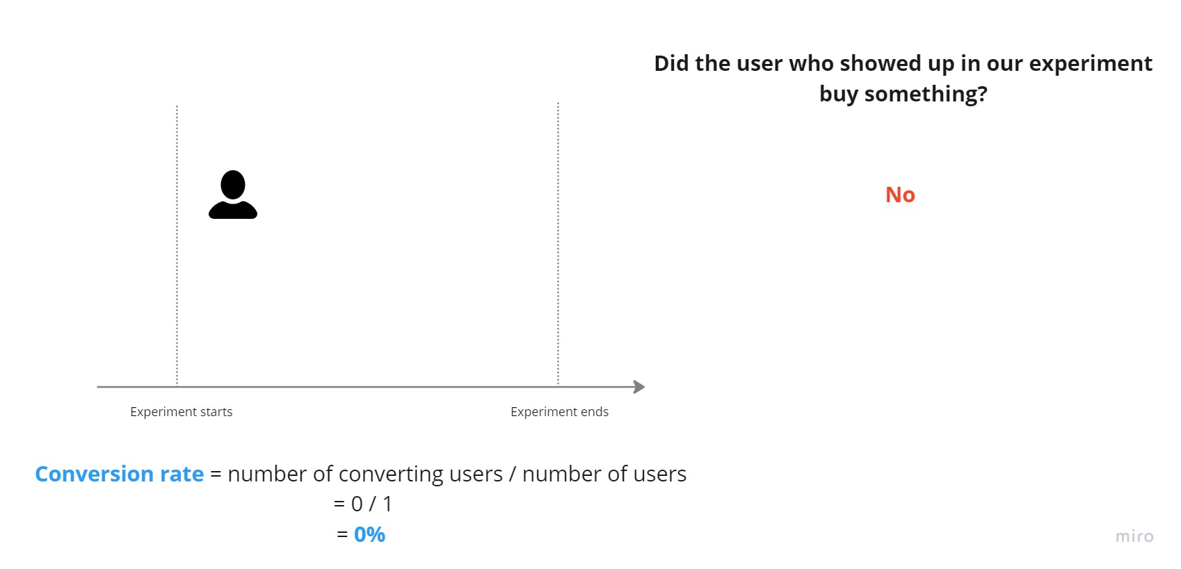
\[\text{Variant group conversion rate} = \frac{\text{Number of unique converting users in our variant group}}{\text{Number of unique users in our variant group}}\]

Let’s illustrate our conversion rate. Here is a timeline of an experiment:

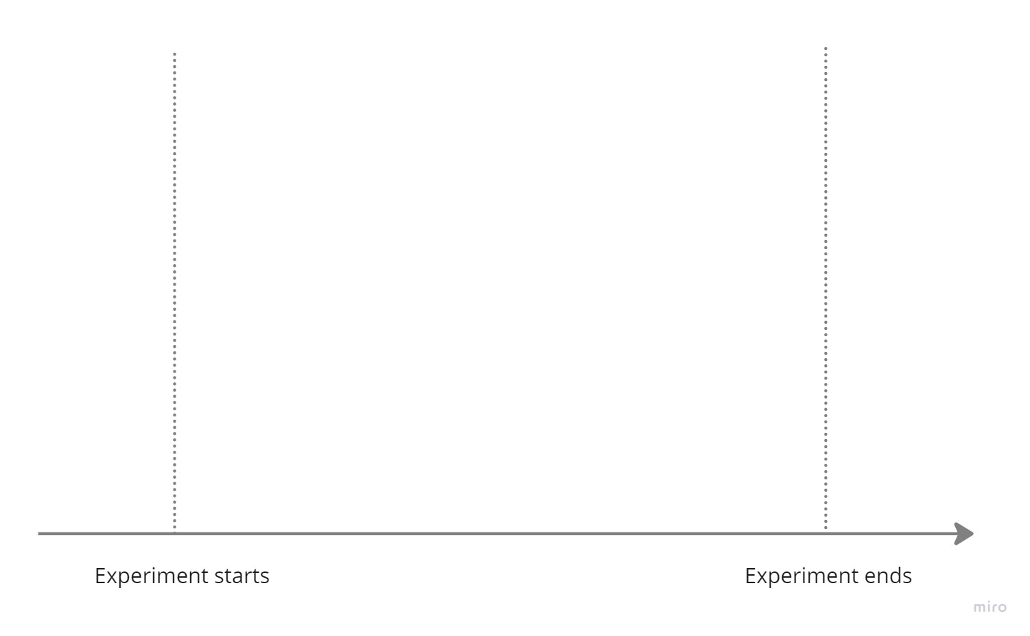
A user shows up in our experiment. They haven’t bought anything yet, so the conversion rate is 0%:

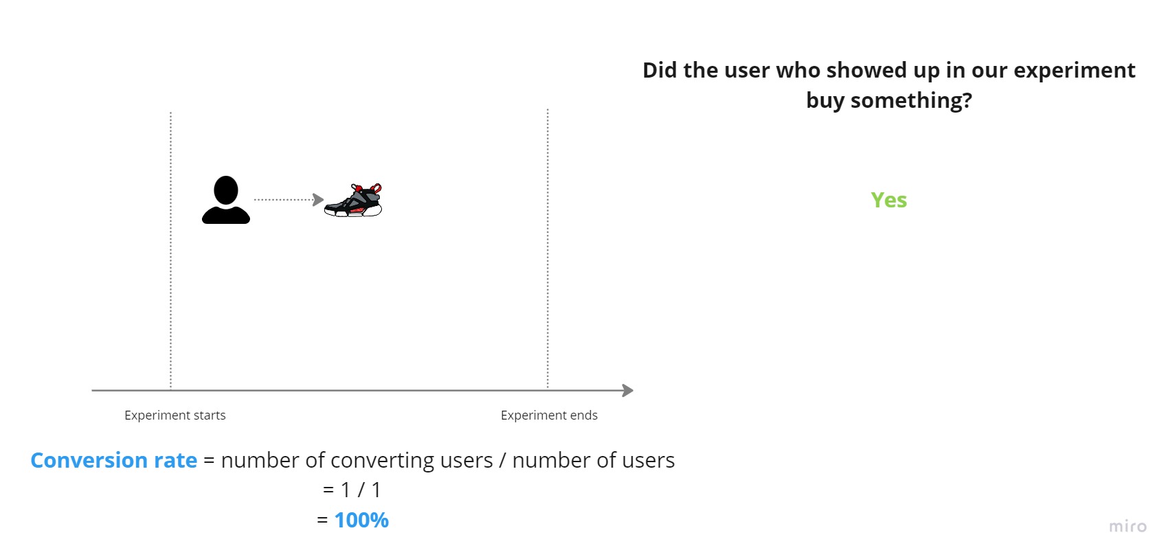
Hooray! The user bought a pair of sweet, sweet sneakers. The conversion rate is now 100%:

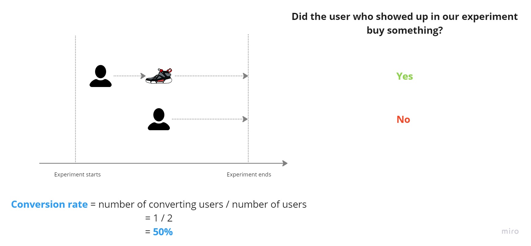
A second user shows up in our experiment. They unfortunately don’t buy anything and the experiment ends. The conversion rate is 50% for the experiment:

How will we measure the “outperformance” of our new algorithm over the existing one?

We have two groups with an equal number of randomly assigned users. We now have two conversion rates:

How can we distil these two rates into a single metric that can be used to describe the difference in performance between the two algorithms? That’s easy!

What we’re interested in is the difference in conversion rates between these groups. Let’s calculate the difference in conversion rates in the above scenario:

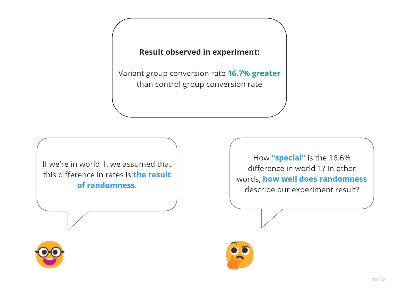
\[\begin{align*} \text{Difference in conversion rates} &= \text{Variant conversion rate} - \text{Control conversion rate} \\ &\approx 66.7\% - 50.0\% \\ &\approx 16.7\% \end{align*}\]

Wow, a +~16.7% absolute difference to control! That’s a relative change of \(\frac{16.7\%}{50\%} \approx ~33.3\%\)!!!

Is the difference in conversion rates just random noise?

We have a +~16.7% absolute difference in conversion rates. It looks like our variant algorithm performs better! We have a winner! Let’s release this to production. Right? Right?

No! Not yet. Let’s dive head-first into the rabbit hole.

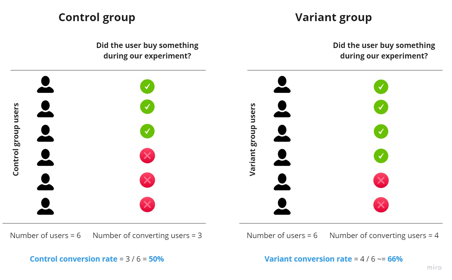
We can’t include all current and all future users in our experiment. That’s impossible! We’re constrained by reality. In our experiment, we’ve only sampled 12 users in total, 6 of whom were randomly assigned to the control group, and 6 of whom were randomly assigned to the variant group.

By only sampling 12 users from a hypothetically infinite group of users, there’s some randomness in which users show up during our experiment. Furthermore, even though we’ve randomly allocated users to the control and variant groups, there’s a naturally random variation in how users behave within each group.

This means our conversion rate measurements are “tinged with randomness”. Oh, beautiful randomness.

Our job is to make an intelligent guess from our limited experiment users whether what we’ve observed is a random blip in outperformance, or whether it could be “true outperformance”.

On our parallel worlds

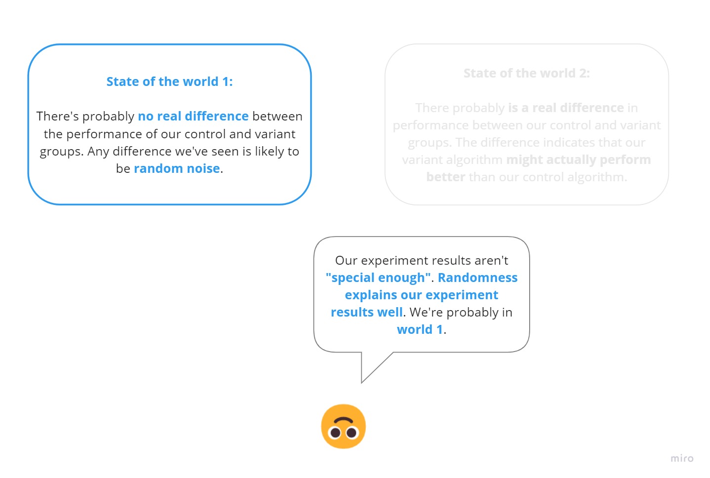
We have two competing states of the world that describe our observed difference in conversion rates:

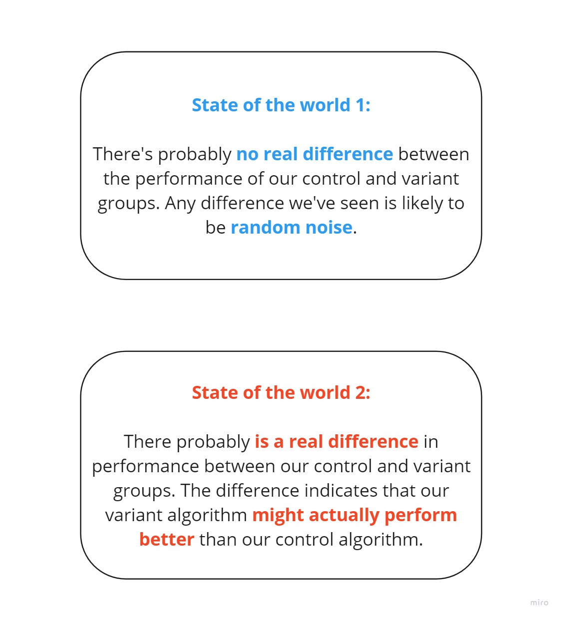
We don’t know which state of the world we’re in. We need to infer which state of the world best describes our experiment results.

Our reasoning process

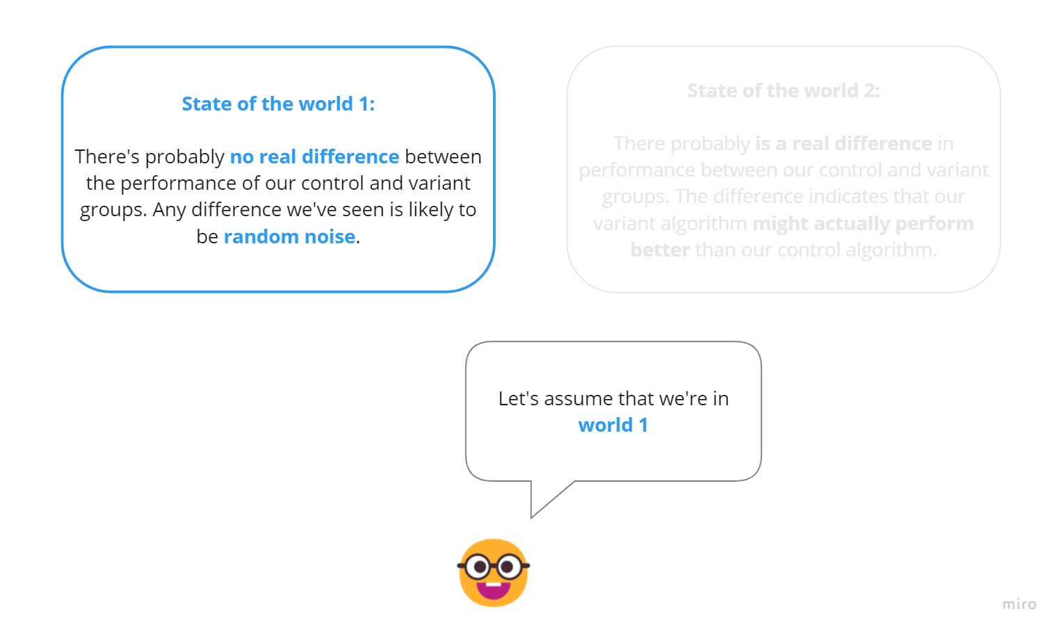
We reason in a reversed way.

We firstly assume we’re in World 1:

We consider our experiment results and how special they are in World 1. We can think of this as answering the question “How out of place are our experiment results if we’re in a world where randomness might have caused our experiment results?”:

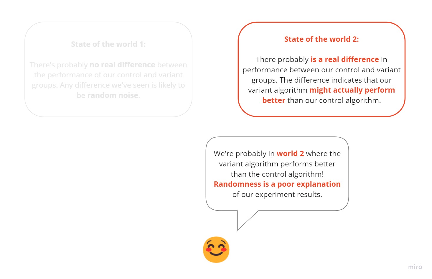
If the experiment results are special enough (i.e. they’re rare in a world where randomness might have caused the results we’ve observed), we say that randomness is a poor descriptor of our experiment results. We conclude that there’s good evidence that our variant algorithm performs better than our control algorithm:

If the experiment results aren’t special enough, we conclude that there’s not enough evidence to say that the variant algorithm performs better than the control algorithm:

On quantifying how well randomness explains our results

How can we quantify how special or not special our experiment result of ~16.7% difference in conversion rates really is?

We could come up with a range of differences in conversion rates caused by randomness alone, and see how extreme our result of ~16.7% difference is.
To come up with a range of random variation in the difference in rates, we can use simulations by “injecting randomness” into our experiment results!
We’ll inject randomness into our experiment results by randomly shuffling our users and creating many different control and variant groups. The key is that we’re randomly shuffling our users. It’s like we’re shuffling a deck of cards. This is pure randomness!

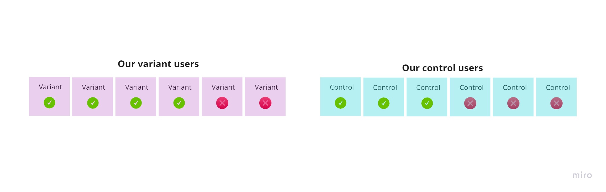
Here are our users from the above artificial experiment, indicating whether they converted or didn’t convert during our experiment:

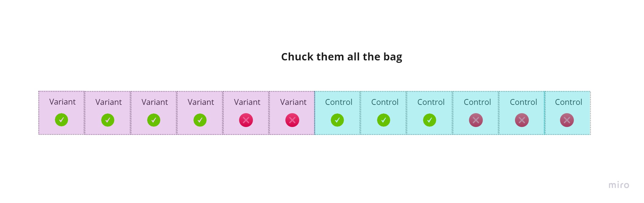
We’re going to chuck our users into a bag. Let’s create our “bag”:

Let’s do the “chucking”:

Let’s randomly shuffle our users:

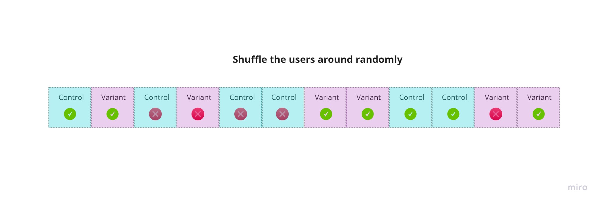
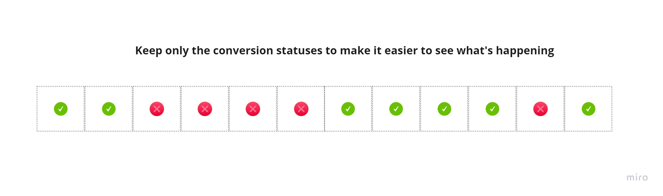
From here on, we’ll keep only our users’ conversion statuses so that it’s easier to understand:

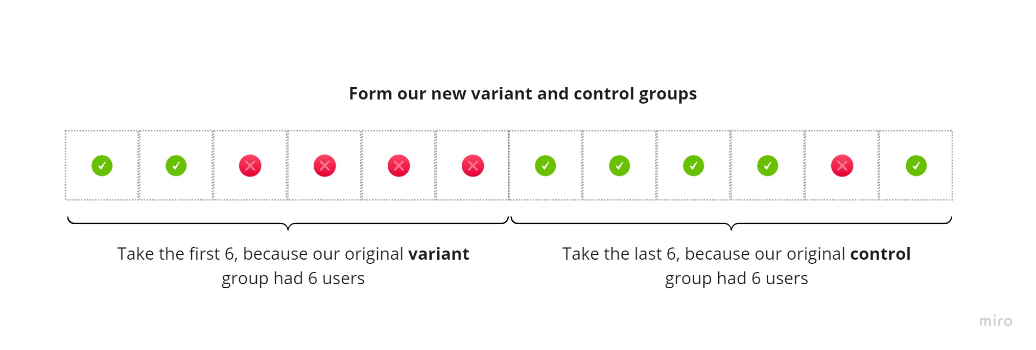
We’ll take the first 6 users and call this our “simulated variant group created by pure randomness”. We’ll take the next 6 users and call this our “simulated control group created by pure randomness”:

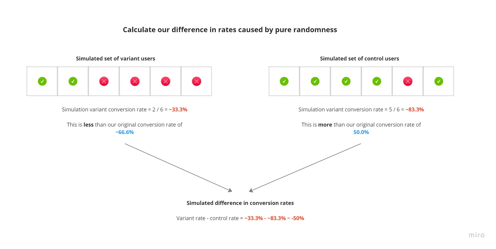
We then calculate our difference in rates between our simulated control and variant groups caused by “pure randomness”:

We repeat this process many times to get a distribution of pure randomness and see where our observed difference of ~16.7% lies.

Now, onto Python!

Creating our range of pure randomness in Python

We’ll be using these techniques for the rest of the post.

Let’s create an array that represents users in our control group and whether the user at that position in the array converted or not. We’re dealing with binary outcomes (the user either converts or not):

A user who converted will be given the value 1
A user who didn’t convert will be given the value 0

NUM_CONTROL_USERS = 6 # total number of users in control group

We’ll create an array in which each index represents a user in our control group:

control_users = np.zeros(NUM_CONTROL_USERS)

control_users

array([0., 0., 0., 0., 0., 0.])

We’ll set the converting users to 1’s:

NUM_CONVERTING_CONTROL_USERS = 3
control_users[:NUM_CONVERTING_CONTROL_USERS] = 1.0

control_users

array([1., 1., 1., 0., 0., 0.])

What’s our control conversion rate?

control_conversion_rate = control_users.mean()
print(f"control conversion rate: {control_conversion_rate:.1%}")

control conversion rate: 50.0%

We’ll do the same for our variant group users:

NUM_VARIANT_USERS = 6
NUM_CONVERTING_VARIANT_USERS = 4

variant_users = np.zeros(NUM_VARIANT_USERS)
variant_users[:NUM_CONVERTING_VARIANT_USERS] = 1.0

variant_conversion_rate = variant_users.mean()
print(f"variant conversion rate: {variant_conversion_rate:.1%}")

variant conversion rate: 66.7%

The difference in rates we saw in our experiment is this:

observed_diff_in_rates = variant_conversion_rate - control_conversion_rate
print(f"observed difference in conversion rates: {observed_diff_in_rates:.1%}")

observed difference in conversion rates: 16.7%

Very good!

Let’s run one iteration of our simulation. Let’s chuck our control and variant users into a bag:

all_users = np.hstack([control_users, variant_users])

all_users

array([1., 1., 1., 0., 0., 0., 1., 1., 1., 1., 0., 0.])

Let’s randomly shuffle them:

rng.shuffle(all_users)

all_users

array([0., 1., 1., 0., 1., 1., 1., 0., 0., 0., 1., 1.])

We create our simulated control and variant groups:

simulated_control_group = all_users[:NUM_CONTROL_USERS]
simulated_variant_group = all_users[NUM_CONTROL_USERS:]

simulated_control_group, simulated_variant_group

(array([0., 1., 1., 0., 1., 1.]), array([1., 0., 0., 0., 1., 1.]))

What are our simulated conversion rates?

print(f"simulated control conversion rate: {simulated_control_group.mean():.1%}")
print(f"simulated variant conversion rate: {simulated_variant_group.mean():.1%}")

simulated control conversion rate: 66.7%
simulated variant conversion rate: 50.0%

simulated_diff_in_rates = simulated_variant_group.mean() - simulated_control_group.mean()

print(f"simulated difference in conversion rates: {simulated_diff_in_rates:.1%}")

simulated difference in conversion rates: -16.7%

Not quite our result of ~+16.7%, is it?

Let’s do this many times:

NUM_SIMULATIONS = 10_000
simulated_diffs_in_rates = []

for _ in range(NUM_SIMULATIONS):
    rng.shuffle(all_users)
    control_conversion_rate = all_users[:NUM_CONTROL_USERS].mean()
    variant_conversion_rate = all_users[NUM_CONTROL_USERS:].mean()
    simulated_diffs_in_rates.append(variant_conversion_rate - control_conversion_rate)

simulated_diffs_in_rates = np.array(simulated_diffs_in_rates)

Let’s inspect our first 10 simulated difference in rates:

for i, rate in enumerate(simulated_diffs_in_rates[:10]):
    print(f"simulated diff in rates {i+1}: {rate:.1%}")

simulated diff in rates 1: -50.0%
simulated diff in rates 2: -16.7%
simulated diff in rates 3: 16.7%
simulated diff in rates 4: 16.7%
simulated diff in rates 5: 50.0%
simulated diff in rates 6: 50.0%
simulated diff in rates 7: -16.7%
simulated diff in rates 8: -16.7%
simulated diff in rates 9: -50.0%
simulated diff in rates 10: 16.7%

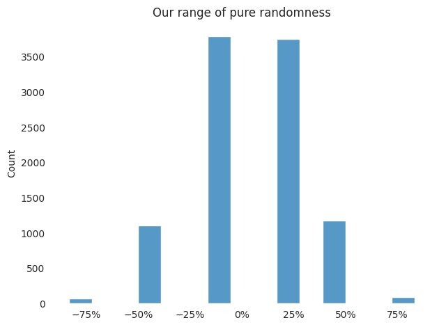
Let’s plot our distribution of pure randomness. This is our distribution of random noise!

Note: we’re dealing with extremely small sample sizes so the distribution ain’t pretty. We’ll be running a large-scale fake example next.

def plot_hist(experiment_results: np.ndarray,
              bins=100,
              observed_rate: float = None,
              title: str = None) -> None:
    sns.histplot(experiment_results, bins=bins)
    if observed_rate:
        plt.axvline(observed_rate, color='r', label='Diff in rates observed in experiment')
        plt.legend(bbox_to_anchor=(0.5, -0.2), loc="lower center")
    if title:
        plt.title(title)
    plt.gca().xaxis.set_major_formatter(ticker.PercentFormatter(xmax=1.0))
    sns.despine(left=True, bottom=True)
    plt.tight_layout()


plot_hist(simulated_diffs_in_rates,
          bins=15,
          title="Our range of pure randomness")

How “special” are our experiment results? On statistical significance

Let’s now infer which world we’re in. Let’s recap our reasoning process:

If our observed experiment result of ~+16.7% “isn’t special enough”, we’re probably in World 1. This is the world where we assume that our experiment result is probably due to random chance. We conclude that, given our experiment, there’s insufficient evidence to say that our variant algorithm performs better than our control algorithm.
If our experiment result “is special enough”, then we’re probably in World 2. This is the world where random chance isn’t a good description for our observed experiment result of ~+16.7%. We conclude that, given our experiment, there’s strong evidence to suggest that our variant algorithm performs better than our control algorithm.

Let’s restate our phrases “isn’t special” and “special” in the context of our distribution of random noise:

If it’s “common” to see an experiment result greater than or equal to ~+16.7% in our distribution of random noise, then our result “isn’t special”. This means that random noise explains our experiment results well.
If it’s “rare” to see an experiment result greater than or equal to ~+16.7% in our distribution of random noise, then our result is “special”. This means that random noise doesn’t explain our experiment results well.

We can now address the “enough” part of the phrases “isn’t special enough” and “is special enough”. The most common threshold of “specialness” used is 5%. What does this mean in our context?

If more than 5% of our randomly generated differences in conversion rates are greater than or equal to our observed experiment result of ~+16.7%, then we say that our experiment result “isn’t special enough”.
- We conclude that the difference in performance we’ve seen is probably just some random noise and that there’s probably no difference in performance.
- We conclude that our result “is not statistically significant”.
If 5% or less of our randomly generated differences in conversion rates are greater than or equal to our observed experiment result of ~+16.7%, then we say that our experiment result “is special enough”.
- We conclude that our experiment result is unlikely to be random noise and that there’s enough evidence that the variant algorithm performs better than our control algorithm.
- We conclude that our result is statistically significant.

Let’s see the above paragraphs in action. Where do our experiment results lie in our distribution of random noise?

plot_hist(simulated_diffs_in_rates,
          bins=15,
          observed_rate=0.167,
          title="Our range of pure randomness")

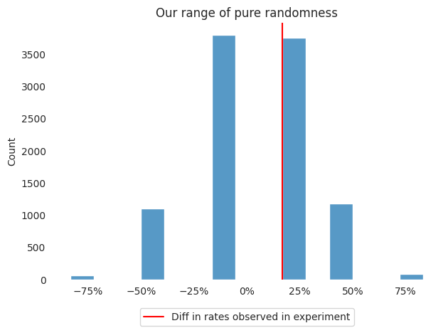
Looking to the right of our red line, we can see the observations that are greater than or equal to our observed result of ~+16.7%. It already looks like more than 5% of our randomly generated differences in conversion rates are >= ~+16.7%. But let’s confirm!

OBSERVED_DIFF_IN_RATES = 0.167 # this is our experiment result

num_diffs_gte_observed = (simulated_diffs_in_rates >= OBSERVED_DIFF_IN_RATES).sum()
num_samples = simulated_diffs_in_rates.shape[0]

print(f"{num_diffs_gte_observed:,} out of {num_samples:,} random samples show differences in rates greater than or equal to {OBSERVED_DIFF_IN_RATES:.1%}")
print(f"percentage of random noise distribution with difference in rates greater than or equal to {OBSERVED_DIFF_IN_RATES:.1%}: {num_diffs_gte_observed / num_samples:.2%}")

1,267 out of 10,000 random samples show differences in rates greater than or equal to 16.7%
percentage of random noise distribution with difference in rates greater than or equal to 16.7%: 12.67%

Now to conclude:

~12.67% of our random samples are greater than or equal to our observed experiment result of ~+16.7%
We hoped that 5% or less of our random samples would be greater than or equal to our observed experiment result of ~+16.7%.
Our experiment result “isn’t special enough”. In other words, our result “is not statistically significant”.
Given how we’ve set up our experiment, our result is probably due to random noise.
We don’t have enough evidence to say that our variant algorithm performs better than our control algorithm.

Nice!

An example where our results are “special enough”

To wrap this up, let’s simulate an example where the difference in performance is “special enough” and we therefore conclude that our variant algorithm might perform better than our control algorithm.

Let’s create a larger fake experiment:

NUM_CONTROL_USERS = 1_000_000
NUM_CONVERTING_CONTROL_USERS = 26_000

NUM_VARIANT_USERS = 1_000_000
NUM_CONVERTING_VARIANT_USERS = 26_400

# create our arrays of users
control_users = np.zeros(NUM_CONTROL_USERS)
control_users[:NUM_CONVERTING_CONTROL_USERS] = 1.0
control_conversion_rate = control_users.mean()

variant_users = np.zeros(NUM_VARIANT_USERS)
variant_users[:NUM_CONVERTING_VARIANT_USERS] = 1.0
variant_conversion_rate = variant_users.mean()

# calculate our experiment result
observed_diff_in_rates = variant_conversion_rate - control_conversion_rate

# chuck our users into a bag
all_users = np.hstack([control_users, variant_users])

print(f"control conversion rate = {control_conversion_rate:.2%}")
print(f"variant conversion rate = {variant_conversion_rate:.2%}")
print(f"observed absolute difference in conversion rates = {observed_diff_in_rates:.2%}")
print(f"observed relative difference in conversion rates = {observed_diff_in_rates / control_conversion_rate:.2%}")

control conversion rate = 2.60%
variant conversion rate = 2.64%
observed absolute difference in conversion rates = 0.04%
observed relative difference in conversion rates = 1.54%

We’ll use the numba library to do the resampling efficiently:

@njit(parallel=True)
def sample_diffs_in_rates(all_users, num_control_users, num_simulations):
    results = np.zeros(num_simulations)
    for i in prange(num_simulations):
        # numpy random shuffling appears to be slower when using numba
        random.shuffle(all_users)
        control_rate = all_users[:num_control_users].mean()
        # we assume the rest of the users are variant users
        variant_rate = all_users[num_control_users:].mean()
        results[i] = variant_rate - control_rate
    return results

Run the simulations!

NUM_SIMULATIONS = 10_000

sampled_diffs = sample_diffs_in_rates(all_users, NUM_CONTROL_USERS, NUM_SIMULATIONS)

Let’s look at where our observed difference of 0.04% lies in our range of randomness:

plot_hist(sampled_diffs,
          bins=50,
          observed_rate=observed_diff_in_rates,
          title="Our range of pure randomness")

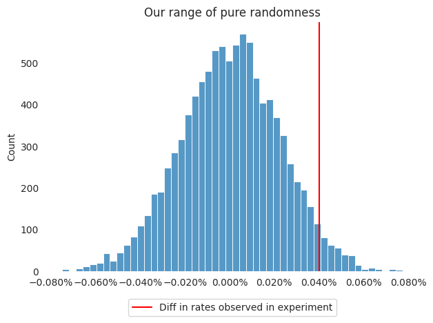
Given our “specialness threshold” of 5%, how well does randomness describe our experiment results?

sampling_specialness_result = (sampled_diffs >= observed_diff_in_rates).sum() / sampled_diffs.shape[0]
print(f"sampled 'specialness' result: {sampling_specialness_result:.2%}")

sampled 'specialness' result: 3.41%

That’s less than 5%! We have a special, statistically significant result. Our variant algorithm probably performs better than our control one.

Let’s compare this to the “actual” result as derived through traditional statistics:

actual_specialness_result = score_test_proportions_2indep(NUM_CONVERTING_VARIANT_USERS, NUM_VARIANT_USERS, NUM_CONVERTING_CONTROL_USERS, NUM_CONTROL_USERS, alternative="larger")
print(f"actual 'specialness' result: {actual_specialness_result.pvalue:.2%}")

actual 'specialness' result: 3.83%

We also have a statistically significant result.

The “specialness” values aren’t equal because they’re derived in different ways. However, they’re close enough for the day-to-day of data scientists. What’s more important is that you specify your “specialness threshold” before running an experiment and stick to it when making decisions based on your experiment’s results.

A note for if you’re doing this at work

You shouldn’t implement this stuff from scratch. Use a robust implementation like the one in scipy.

Phew! We’re done!

Justin

Faster web scraping with Python and asyncio

2023-02-11T12:39:00+11:00

Do you use Jupyter? Are you still sending sequential web requests like a noob? Then this article is for you!

This article is for intermediate Python programmers, so I’m going to skip over a lot of the detail.

I couldn’t have done this without these two books:

Python Concurrency with asyncio by Matthew Fowler

Using Asyncio in Python: Understanding Python’s Asynchronous Programming Features by Caleb Hattingh

These books are great. Buy them!

Packages used in this post

# standard library packages
import asyncio 
import gzip 
import functools 
from functools import partial 
from time import perf_counter
import random

# other packages
import requests
import aiohttp

Getting some data to work with

We’ll be using a sample file from the Wikimedia dumps:

WIKIMEDIA_DUMP_URL = "https://dumps.wikimedia.org/enwiki/latest/enwiki-latest-all-titles.gz"

response = requests.get(WIKIMEDIA_DUMP_URL)

The file is a gzip file, so we need to decompress it. gzip.decompress returns a byte string that can be decoded to UTF-8:

titles = gzip.decompress(response.content).decode("utf-8")

Let’s take a look at our data. There are some interesting article titles here. I’m leaving them in for science! No need to hide them.

titles[:100]

'page_namespace\tpage_title\n0\t!\n0\t!!\n0\t!!!\n0\t!!!!!!!\n0\t!!!Fuck_You!!!\n0\t!!!Fuck_You!!!_And_Then_Some\n0'

We make some observations:

We’ve got one huge string
There’s a header row, indicating there are two columns: page_namespace and page_title
The file is tab-delimited, indicated by the \t characters
There are new line characters, indicated by the \n characters

I don’t want to process this whole string for this demonstration. Let’s take the first 100k article titles:

num_new_lines = 0
for i in range(len(titles)):
    if titles[i] == "\n":
        num_new_lines += 1
    # we add 1 to the number of lines to account for the header row
    if num_new_lines >= 100_000 + 1:
        target_index = i
        break    

This is the position of the new line character immediately after the 100,000th article title:

print(target_index)

titles_substr = titles[:target_index]

Next, we extract the article titles. We’ll do these things:

Split the string on new line characters
Split each line by the tab delimiter and take the second element, which is the article title
Remove the first element to discard the header row

titles_sample = [line.split('\t')[1] for line in titles_substr.split('\n')]
titles_sample = titles_sample[1:]

The result is a list of 100k article titles:

titles_sample[:10]

['!',
 '!!',
 '!!!',
 '!!!!!!!',
 '!!!Fuck_You!!!',
 '!!!Fuck_You!!!_And_Then_Some',
 '!!!Fuck_You!!!_and_Then_Some',
 '!!!_(!!!_album)',
 '!!!_(American_band)',
 '!!!_(Chk_Chk_Chk)']

print(f"number of article titles: {len(titles_sample):,}")

number of article titles: 100,000

Noice!

Making the requests

We’ll be making the request to URLs looking like this:

WIKIPEDIA_BASE_URL = "https://en.wikipedia.org/wiki/{TITLE}"

Here’s the first URL:

title = titles_sample[0]
url = WIKIPEDIA_BASE_URL.format(TITLE=title)
print(url)

https://en.wikipedia.org/wiki/!

Let’s make a single request:

response = requests.get(url)

The response is a byte string, so we’ll decode it to UTF-8:

response.content.decode('utf-8')[:1000]

'\n\n\n\nExclamation mark - Wikipedia\n

Waking up at 4:00 AM just to do more stuff? Go back to sleep if that’s not how your body works or if you don’t have a good reason to wake up at that time.

Listening to your audiobook at 300% speed to absorb ideas “TO THE MAX”? Bleugh! Just enjoy the damn book!

Oliver Burkeman’s “Four Thousand Weeks”

This book has, so far, been amazing. It’ll help you live a more fulfilling life. The key ideas have so far been these:


  We try to manage our time to get the most out of our days in the hope that once we get through the tasks on our ever-growing-to-do lists, we will finally get what is truly important to us.
  The paradox is that the more efficient we get at clearing our lists and our inboxes, the more stuff appears to fill it.
  We avoid facing the reality that our time on this earth is frighteningly short by fooling ourselves that we have time to work on everything because this means that we don’t have to make difficult trade-offs as to how we choose to use our time. We fool ourselves by thinking that with enough hard work, we can make all of our dreams come true and that we’re capable of doing everything.
  Others can make impossible demands on your time by asking you to do so many things that it’s simply not possible to do them all. You might be the one making these impossible demands on your time. Once you accept that these demands are in fact impossible, you empower yourself to resist them.
  We should embrace our own limits. We simply don’t have the time to do all of the things we want to do. We might not have the talent required to do some things. We also don’t have the time to do all the things others want us to do. So we shouldn’t beat ourselves up over it!
  Making a choice to spend your time on something inevitably means that you’re choosing not to spend your time doing something else. The important thing is that you’re making a conscious choice and not letting others make that choice for you.


One of my favourite quotes so far is this one from page 30:


  Every decision to use a portion of time on anything
represents the sacrifice of all the other ways in which you
could have spent that time, but didn’t—and to willingly make
that sacrifice is to take a stand, without reservation, on what
matters most to you.


How am I applying what I’ve learned so far to my own life?

This book has allowed me to reflect on a few aspects of my life:

  I probably will never finish my Master’s in computing because it takes up too much of my time and energy. I really love learning about computers, networking, algorithms etc. But I don’t need to go to uni to learn these things. Formal studies detract from my ability to do the things I love, like spending time with my family, hiking and learning and writing about random things just because they’ve captivated my imagination.
  As a result, I will probably never get a PhD in computing or AI. This would mean subjecting myself to years of hard work and taking a big pay cut, which will detract from my ability to take care of my aging mum and build a life of adventure together with my wife (who I love very much).
  I will probably never live and work in Silicon Valley. Making this dream come true would mean trading off a lot of things: time spent with my loved ones in Australia and working my ass off in the Mecca of hustle culture.


Choosing not to do the above means I choose to spend my time on the things that mean a lot to me:

  Hiking with my wife
  Spending time with my mum
  Reading books because I want to and not because I need to read a prescribed textbook for uni
  Saying “yes” to more social engagements, and not saying “no” because I need to study for an upcoming exam
  Living in another country for a few months whenever we choose to because I don’t have to be back in the country to take an exam


The above choices feel good and I will have to remind myself to reassess the things that matter to me most again a few years down the track.

Some choice quotes

From page 11:


  It follows from this that time management, broadly defined,
should be everyone’s chief concern. Arguably, time management
is all life is. Yet the modern discipline known as time
management—like its hipper cousin, productivity—is a
depressingly narrow-minded affair, focused on how to crank
through as many work tasks as possible, or on devising the
perfect morning routine, or on cooking all your dinners for the
week in one big batch on Sundays.


From page 14:


  In the modern
world, the American anthropologist Edward T. Hall once pointed
out, time feels like an unstoppable conveyor belt, bringing us
new tasks as fast as we can dispatch the old ones; and
becoming “more productive” just seems to cause the belt to
speed up.


From page 16:


  Our days are spent trying to “get through” tasks,
in order to get them “out of the way,” with the result that we
live mentally in the future, waiting for when we’ll finally get
around to what really matters—and worrying, in the meantime,
that we don’t measure up, that we might lack the drive or
stamina to keep pace with the speed at which life now seems
to move.


From page 17:


  Productivity is a trap. Becoming more efficient
just makes you more rushed, and trying to clear the decks
simply makes them fill up again faster. Nobody in the history
of humanity has ever achieved “work-life balance,” whatever
that might be, and you certainly won’t get there by copying the
“six things successful people do before 7:00 a.m.”


From page 24:


  Once time
is a resource to be used, you start to feel pressure, whether
from external forces or from yourself, to use it well, and to
berate yourself when you feel you’ve wasted it. When you’re
faced with too many demands, it’s easy to assume that the
only answer must be to make better use of time, by becoming
more efficient, driving yourself harder, or working for longer—as
if you were a machine in the Industrial Revolution—instead of
asking whether the demands themselves might be unreasonable.


From pages 24-25:


  The fundamental problem is that this attitude toward time sets
up a rigged game in which it’s impossible ever to feel as
though you’re doing well enough. Instead of simply living our
lives as they unfold in time—instead of just being time, you
might say—it becomes difficult not to value each moment
primarily according to its usefulness for some future goal, or
for some future oasis of relaxation you hope to reach once your tasks are finally “out of the way.”


From page 28:


  After all, it’s painful to confront how limited your
time is, because it means that tough choices are inevitable and
that you won’t have time for all you once dreamed you might
do. It’s also painful to accept your limited control over the time
you do get: maybe you simply lack the stamina or talent or
other resources to perform well in all the roles you feel you
should. And so, rather than face our limitations, we engage in
avoidance strategies, in an effort to carry on feeling limitless.
We push ourselves harder, chasing fantasies of the perfect
work-life balance; or we implement time management systems
that promise to make time for everything, so that tough choices
won’t be required. Or we procrastinate, which is another means
of maintaining the feeling of omnipotent control over
life—because you needn’t risk the upsetting experience of failing
at an intimidating project, obviously, if you never even start it.


From page 30:


  In practical terms, a limit-embracing attitude to time means
organizing your days with the understanding that you definitely
won’t have time for everything you want to do, or that other
people want you to do—and so, at the very least, you can stop
beating yourself up for failing. Since hard choices are
unavoidable, what matters is learning to make them consciously,
deciding what to focus on and what to neglect, rather than
letting them get made by default—or deceiving yourself that,
with enough hard work and the right time management tricks,
you might not have to make them at all.


Take the antidote

There’s a lot to ponder here. Take the antidote and count yourself out of the “rise and grind” culture. Read the book!

Justin



Docker and Makefiles
2022-08-07T08:29:00+10:00

  A whale of a time!


I’m learning PyTorch!

I’m writing a Dockerfile using a PyTorch base image and installing some Python packages that’ll be useful when developing my models.

I use Makefiles a lot to make my Docker-based workflows easier. I stumbled across a nice Makefile pattern in the PyTorch repo and wanted to share it with y’all.

The original Makefile

With my simple Dockerfile in the same directory as my Makefile, I started out writing my Makefile like this:

.PHONY: build
build:
	docker build --progress=plain -t pytorch .

.PHONY: check-gpu
check-gpu:
	docker run --rm --gpus all pytorch nvidia-smi

.PHONY: bash
bash:
    docker run --rm --gpus all pytorch bash


The PyTorch Makefile pattern

In my journey into the PyTorch repo, I found this Makefile, which is used in the build_publish_nightly_docker.sh script.

It extracts the docker build and docker push commands into the DOCKER_BUILD and DOCKER_PUSH Makefile variables:

DOCKER_BUILD  = DOCKER_BUILDKIT=1 \
		docker build \
			--progress=$(BUILD_PROGRESS) \
			$(EXTRA_DOCKER_BUILD_FLAGS) \
			--target $(BUILD_TYPE) \
			-t $(DOCKER_FULL_NAME):$(DOCKER_TAG) \
			$(BUILD_ARGS) .
DOCKER_PUSH = docker push $(DOCKER_FULL_NAME):$(DOCKER_TAG)


It also extracts Docker build args into their own variable:

BUILD_ARGS  = --build-arg BASE_IMAGE=$(BASE_IMAGE) \
		--build-arg PYTHON_VERSION=$(PYTHON_VERSION) \
		--build-arg CUDA_VERSION=$(CUDA_VERSION) \
		--build-arg CUDA_CHANNEL=$(CUDA_CHANNEL) \
		--build-arg PYTORCH_VERSION=$(PYTORCH_VERSION) \
		--build-arg INSTALL_CHANNEL=$(INSTALL_CHANNEL)


To build and push the Docker images, other Makefile targets make use of  the above variables. In subsequent Makefile targets, some build args are replaced before executing the command contained within the DOCKER_BUILD and DOCKER_PUSH variables:

runtime-image: BASE_IMAGE := $(BASE_RUNTIME)
runtime-image: DOCKER_TAG := $(PYTORCH_VERSION)-runtime
runtime-image:
	$(DOCKER_BUILD)
	docker tag $(DOCKER_FULL_NAME):$(DOCKER_TAG) $(DOCKER_FULL_NAME):latest

runtime-push: BASE_IMAGE := $(BASE_RUNTIME)
runtime-push: DOCKER_TAG := $(PYTORCH_VERSION)-runtime
runtime-push:
	$(DOCKER_PUSH)


My new Makefile

My Makefile is far simpler than the PyTorch one. However, thanks to their Makefile pattern, my simple Makefile is a little bit cleaner and a little bit more maintainable:

IMAGE_TAG = pytorch
INTERACTIVE = 
DOCKER_RUN = docker run \
		--rm \
		--gpus all \
		$(INTERACTIVE) \
		$(IMAGE_TAG)

.PHONY: build
build:
	docker build --progress=plain -t $(IMAGE_TAG) .

.PHONY: check-gpu
check-gpu:
	$(DOCKER_RUN) nvidia-smi

.PHONY: bash
bash: INTERACTIVE := -it
bash:
	$(DOCKER_RUN) bash	


Thank you, PyTorch maintainers!

Justin


Render LaTeX in Google Docs
2021-09-23T08:11:00+10:00

  This is for all the students out there!


It turns out that a Google image search for the word “latex” returns many not-safe-for-work images. That’s not the sort of “latex” I’m talking about!

What I’m talking about here is the famous typesetting system, \(\LaTeX\). If you study anything technical at university (or college for readers in the US who seem to make up the majority of my readers!), you would have come across it.

I use Google Docs a lot. I use it at university, at work, and in my personal life. Being a nerd, I frequently need to write equations in Google Docs. Is there a way to write \(\LaTeX\) equations in Google Docs?

Yes, there most certainly is!

How to write and render LaTeX in Google Docs

Install “Auto-LaTeX Equations”


  Open up Google Docs and create a new document.
  Go to “Add-ons” -> “Get add-ons”





  Search for the word “latex”. The first result should be “Auto-LaTeX Equations. Install it!





  Once installed, go back to “Add-ons” -> “Auto-LaTeX Equations” -> “Start”




The Auto-LaTeX Equations toolbar should appear on the right-hand side of the screen.



Noice.

Writing single-line equations

Just wrap what you want to render into Latex in double dollar signs.



Then click on “Render Equations”.



After a little while, you should see something like this!



Nooooooice.

Writing multi-line equations


  Start with two dollar signs, just like with single-line equations. Press shift + enter.
  Type the LaTeX for your first equation. Press shift + enter.
  Type the LaTeX for your second equation. Press shift + enter.
  Type the LaTex for your \(n\)th equation. Press shift + enter.
  Type two dollar signs.
  Press “Render Equations”


Something like this:



will turn into this:



Noooooooooooooooice.

How to write some mathematical things using LaTeX

Here’s a brain dump of things I commonly use.

Fractions

\frac{1}{2} gives you \(\frac{1}{2}\)

Less than, greater than, less than or equal to, greater than or equal to

< gives you \(<\)

> gives you \(>\)

\leq gives you \(\leq\)

\geq gives you \(\geq\)

Exponents and subscripts

x^i gives you \(x^i\)

x^{2n + 1} gives you \(x^{2n + 1}\)

x_{i} gives you \(x_{i}\)

x_{2n + 1} gives you \(x_{2n + 1}\)

Approximately

\approx gives you \(\approx\)

Equivalence

\equiv gives you \(\equiv\)

Sums and products

\sum\limits_{i=1}^{n} x_i gives you \(\sum\limits_{i=1}^{n} x_i\)

\prod\limits_{i=1}^{n} x_i gives you \(\prod\limits_{i=1}^{n} x_i\)

Partial derivatives

\frac{\partial}{\partial x} x^2 + 3y gives you \(\frac{\partial}{\partial x} x^2 + 3y\)

Gradient

\nabla f gives you \(\nabla f\)

That dot from one of the ways to depict a dot product

x \cdot y gives you \( x \cdot y \)

Big parentheses and brackets

7\left(\frac{x + y}{2}\right) gives you \(7\left(\frac{x + y}{2}\right)\)

z\left[x^2 + 7y\right] gives you \(z\left[x^2 + 7y\right]\)

Adding text in equations

n\text{th} gives you \(n\text{th}\)

Arrows like “implies”

\to and \rightarrow give you \(\to\)

\leftarrow give you \(\leftarrow\)

\implies gives you \(\implies\)

Greek alphabet

They follow a pattern where the lower case variant of the Greek letter begins with a lower case letter. The upper case variant of the same Greek letter begins with an upper case letter. Here are some examples:

\pi and \Pi give you \(\pi\) and \(\Pi\)

\phi and \Phi give you \(\phi\) and \(\Phi\)

\theta and \Theta give you \(\theta\) and \(\Theta\)

Ellipses

\dots gives you \(\dots\)

Proper subsets and subsets

\subset gives you \(\subset\)

\subseteq gives you \(\subseteq\)

Union, intersection

\cup gives you \(\cup\)

\cap gives you \(\cap\)

Aligning equations

Aligning multi-line equations around equal signs can be done by wrapping it in the align environment. Here’s an example:

\begin{align*}
x &= 20y + z \\
z &= \frac{x}{y}
\end{align*}


\[\begin{align*}
x &= 20y + z \\
z &= \frac{x}{y}
\end{align*}\]

Conclusion

Nooooooooooooooooooooooooooooooooooooooooooooooooooooooooice.

No conclusion, really.

I hope you keep on learning!

Justin


The best bolognese recipe
2021-09-12T08:00:00+10:00

  Well, that was unexpected…


Hello!

It’s been ages since I’ve felt like writing anything here. Yesterday I felt the urge again. So here I am! I have a few unfinished post series I want to eventually complete. It can get a tiring always writing about technical things so I’m going to mix it up from time to time.

My wife and I have been enjoying this bolognese recipe for years. If you like an intense sauce, this one’s for you. I’m going to write a variation of it in a no-nonsense way. Here we go!

Buy


  1 carrot
  1 small onion
  1 garlic clove
  500 grams of your preferred minced meat. I normally go with straight-up beef.
  100 grams of pancetta
  Unsalted butter
  Olive oil
  Salt
  Pepper
  Tomato paste
  400 gram tin of chopped tomatoes
  1 bay leaf
  At least 100 ml of beef stock
  Red wine
  Parmigiano-Reggiano
  375 grams of fresh fettuccine or pappardelle.


Most importantly - no celery. I hate celery!

Prepare


  Dice onions
  Dice carrots
  Mince garlic clove
  Dice pancetta into small cubes
  Grate some Parmigiano-Reggiano. You’ll be sprinking this on top of your portions.


Cook


  Get a medium sized pot. Put it on low-medium heat.
  Add 3 tablespoons of olive oil and 50 grams of butter to pot.
  Once butter is melted, add your panchetta cubes. Cook them until golden.
  Add onions, carrots, garlic clove and bay leaf to the pot. Cook until onions turn translucent.
  Add minced meat. Break it up and season with pepper. Cook until meat is coloured.
  Turn up heat to high. Give it a few minutes to heat up.
  Add red wine. Let it cook for a few minutes until smell of alcohol disappears.
  Reduce heat to low-medium.
  Add 2 tablespoons of tomato puree, the whole tin of chopped tomatoes and 100 ml of beef stock to the pot.
  If you have the time, let the sauce cook for 1 hour. Add a little bit of water if the sauce is drying out. If you’re in a rush, cook until sauce is thickened to your liking.
  Remove sauce from heat and let it rest for 5 mins.
  About 15 mins before your sauce is done, fill the largest pot you can find with water and bring it to a boil. Salt the water heavily once boiling. Cook your pasta to your liking.


Serve


  Strain pasta. Return it to the large pot it was cooked in.
  Pour sauce into the large pot with pasta and mix.
  Serve with heaps of grated Parmigiano-Reggiano.


Done!

Justin


Learning to rank is good for your ML career - Part 2: let’s implement ListNet!
2020-06-07T07:00:00+10:00

  The second post in an epic to learn to rank lists of things!


Introduction

Now that we know something about word embeddings, let’s use them as inputs into a model that ranks things!

We’ll be working through my implementation of a model called ListNet, which was proposed in this paper:


  Cao, Zhe et al. “Learning to rank: from pairwise approach to listwise approach.” ICML ‘07 (2007)


There’ll be a bunch of maths in this post. But don’t worry! We’ll be stepping through it together. I’m here for you!

The setup

Here be our packages for this post.

import random
random.seed(1)

import numpy as np
np.random.seed(1)

import itertools
import matplotlib.pyplot as plt
plt.style.use('ggplot')

import tensorflow as tf


Note: it’s notoriously difficult to make TensorFlow and Keras reproducible.  Randomness plays an important part in training neural networks, after all! You might not get the exact numbers shown once we start using TensorFlow later on in the post. But the outcome that I arrive at should be similar to yours! See this post by fellow Aussie Jason Brownlee for more info on this topic.

Let’s start at the end and break it down

Let’s start with a high-level view of what we want to accomplish with ListNet. We’ll use icons of items of clothing in place of our documents because they’re more visually pleasing than article headlines!

We’re going to give ListNet a query, and a bunch of documents to rank. Then, as if through some sorcery, we get a ranked list of documents:



What magic is involved in producing this ranked list? Prepare to be disappointed - ‘cause it ain’t too complex!

ListNet outputs a bunch of real numbers. Each real number is a score assigned to the document we want to rank. We simply sort the documents in descending order of score, and this tells us how the original list of documents should be ranked!



So how does the paper itself describe ListNet? We find this on page four:


  We employ a new learning method for optimizing the listwise loss function based on top one probability, with Neural Network as model and Gradient Descent as optimization algorithm. We refer to the method as ListNet.


Let’s break this down and attack it’s smaller pieces relentlessly in our usual way!

We’ll attack in this order:


  What do they mean by listwise?

  What is this top one probability they speak of?

  What is the listwise loss function?

  What is the neural network architecture?


If you’ve been reading this, I’ll assume that you know what gradient descent is.

Let’s do this!

What’s a ‘listwise approach’ to learning to rank?

Let’s start with our first question!

There are several approaches to learning to rank. In Li, Hang. (2011). A Short Introduction to Learning to Rank., the author describes three such approaches: pointwise, pairwise and listwise approaches.

On page seven, the author describes listwise approaches:


  The listwise approach addresses the ranking problem in a more straightforward way. Specifically, it takes ranking lists as instances in both learning and prediction. The group structure of ranking is maintained and ranking evaluation measures can be more directly incorporated into the loss functions in learning.


Alright! That’s not too bad. We can make some observations at this point.

Firstly, pointwise and pairwise approaches ignore the group structure of rankings. Lists can be thought of as groups of objects placed in specific orders. It makes sense that if we take a listwise approach that the structure of objects within our list is maintained!

Learning to rank often involves optimising a surrogate loss function. This is because the loss function that we want to optimise for our ranking task may be difficult to minimise because it isn’t continuous and uses sorting! ListNet allows us to construct our ranking task in such a way that decreasing its loss values more directly impacts our “true” objective (for example, increasing Normalised Discounted Cumulative Gain or Mean Average Precision).

First question answered. Tick!

Where do probabilities fit into ListNet?

The authors use a probability-based approach to map their lists of scores to probability distributions. Once this is done, they calculate their loss between the predicted probability distribution and a target probability distribution. The authors describe their rationale for defining the problem in this way on page three:


  We assume that there is uncertainty in the prediction of ranking lists (permutations) using the ranking function. In other words, any permutation is assumed to be possible, but different permutations may have different likelihood calculated based on the ranking function. We define the permutation probability, so that it has desirable properties for representing the likelihood of a permutation (ranking list), given the ranking function.


Very nice! The two probability models described are the permutation and top one probability models. We’ll now go through them in turn.

Warning: detail ahead!

If you’re pragmatic, then I’ll let you in on a secret: the authors end up using the top one probability model so you can skip the section on ‘permutation probability’.

However, if you have a burning desire to understand things from their deepest depths, read on! Let’s flex our mathematical muscles!

Permutation probability

Let’s use the same ‘dress’, ‘shirt’ and ‘pants’ example from above. We have \(n = 3\) objects to rank:

objects_to_rank = {'dress', 'shirt', 'pants'}




What are all the possible permutations of these three objects?

all_permutations = list(itertools.permutations(objects_to_rank))

for x in sorted(all_permutations):
    print(x)


('dress', 'pants', 'shirt')
('dress', 'shirt', 'pants')
('pants', 'dress', 'shirt')
('pants', 'shirt', 'dress')
('shirt', 'dress', 'pants')
('shirt', 'pants', 'dress')




The authors depict this set of possible permutations of \(n\) objects as \(\Omega_n\). The authors depict a single permutation in \(\Omega\) as \(\pi = \langle \pi(1), \pi(2), \dots, \pi(n)\rangle\). Each \(\pi(j)\) denotes the object at position \(j\) in the particular permutation.

Say that each one of these objects is given a real number (a score) by our model which can be used to rank the objects. The authors denote the list of scores associated with each object in a permutation \(\pi\) as \(s = (s_1, s_2, \dots, s_n)\), where each \(s_j\) is the score of the \(j\)-th object.



How can we determine the probability of one of the permutations above, given the ranking function that created these scores?

The authors say that this is how you can do just that:

\[P_s(\pi) = \prod_{j=1}^n \frac{\phi(s_{\pi(j)})}{\sum_{k=j}^n \phi(s_{\pi(k)})}\]

This looks like a lot of stuff! But again I say “don’t be scared”! Let’s break it down into tiny pieces.


  Firstly, what are we calculating? We are calculating the probability of some permutation \(\pi\) given some list of scores \(s\). This is depicted by the LHS of the above by \(P_s(\pi)\).
  Next, we notice the big \(\Pi\). This is capital \(\pi\). This symbol says that we will be calculating the product of \(n\) terms. This will become clearer when we go through an example, below.
  Next, we have some \(\phi\)’s. This is the letter ‘phi’. Here, it’s simply some transformation applied to our scores. The only requirement is that it is “an increasing and strictly positive function”, as mentioned on page three.
  The denominator contains a big \(\Sigma\). It tells us that we will be summing \(n - k + 1\) terms. Each one of these terms is a score transformed by the same function \(\phi\).


Walking through an example will clear things up further! We will depict \(\phi\) as an exponential function just like the authors do. Specifically, we will define it as \(\phi(x) = e^x = exp(x)\).

Let’s randomly generate scores for our three objects:

scores_dict = {x: np.random.randn(1)[0] for x in ['shirt', 'pants', 'dress']}  

print(scores_dict)


{'dress': 1.6243453636632417, 'shirt': -0.6117564136500754, 'pants': -0.5281717522634557}


Let’s pick one of our permutations:

pi = random.choice(all_permutations)

print(pi)


('dress', 'shirt', 'pants')




obj_pos_1, obj_pos_2, obj_pos_3 = pi

print(f"object at position 1 is '{obj_pos_1}'")
print(f"object at position 2 is '{obj_pos_2}'")
print(f"object at position 3 is '{obj_pos_3}'")


object at position 1 is 'dress'
object at position 2 is 'shirt'
object at position 3 is 'pants'


We get the scores of the objects at the above positions in our permutation:

score_obj_pos_1 = scores_dict[obj_pos_1]
score_obj_pos_2 = scores_dict[obj_pos_2]
score_obj_pos_3 = scores_dict[obj_pos_3]


Let’s write out the \(n = 3\) terms in our product explicitly!

This is what our first term is:

\[\text{first term} = \frac{e^{s_{dress}}}{e^{s_{dress}} + e^{s_{pants}} + e^{s_{shirt}}}\]

Evaluating it in Python, we get this:

first_term_numerator = np.exp(score_obj_pos_1)
first_term_denominator = np.exp(score_obj_pos_1) + np.exp(score_obj_pos_2) + np.exp(score_obj_pos_3)

first_term = first_term_numerator / first_term_denominator

print(f"first term is {first_term}")


first term is 0.8176176084739423


According to our formula, this is what our second term is:

\[\text{second term} = \frac{e^{s_{pants}}}{e^{s_{pants}} + e^{s_{shirt}}}\]

Evaluating the second term in Python, we get this:

second_term_numerator = np.exp(score_obj_pos_2)
second_term_denominator = np.exp(score_obj_pos_2) + np.exp(score_obj_pos_3)

second_term = second_term_numerator / second_term_denominator

print(f"second term is {second_term}")


second term is 0.47911599189971854


Finally, the third term is this:

\[\text{third term} = \frac{e^{s_{shirt}}}{e^{s_{shirt}}} = 1\]

We’ll just assign this value to a variable for the third term:

third_term = 1.0


It’s not that bad when you break it down, right? Putting it all together, the probability of our permutation is then this:

\[P_s(\langle \text{dress, shirt, pants} \rangle) = \prod_{j=1}^3 \frac{e^{s_{\pi(j)}}}{\sum_{k=j}^3 e^{s_{\pi(k)}}}\]

This is equivalent to the following:

\[\frac{e^{s_{dress}}}{e^{s_{dress}} + e^{s_{pants}} + e^{s_{shirt}}} \cdot \frac{e^{s_{pants}}}{e^{s_{pants}} + e^{s_{shirt}}} \cdot \frac{e^{s_{shirt}}}{e^{s_{shirt}}}\]

Evaluating this in Python, we get this:

prob_of_permutation = first_term * second_term * third_term

print(f"probability of permutation is {prob_of_permutation}")


probability of permutation is 0.39173367147866855


If we calculate the probability of each permutation in our set, we can see that each one is greater than zero and that they sum to one!



We can make an interesting observation at this point:


  The scores sorted in descending order have the highest permutation probability.

The scores sorted in ascending order have the lowest permutation probability.


Interesting! We’re done with the hardest part!

What’s the issue with calculating permutation probability?

To calculate the difference between our distributions using a listwise loss function, we could first calculate the permutation probability distributions for each training example. But this issue with this approach is that there are \(n!\)  permutations! The number of permutations that need to be calculated quickly gets out of hand.

Instead, the authors propose using another probability model that is based on “top one” probability.

Top one probability

Given some object we want to rank, \(j\), the top one probability for that object is the sum of the permutation probabilities of the permutations where \(j\) is ranked first.

\[P_s(j) = \sum_{\pi(1)=j,\pi \in \Omega_n} P_s(\pi)\]

Given our above example, the top one probability for ‘shirt’ is then \(\approx 0.0783 + 0.0091 = 0.087\).

The authors then observe that to calculate the top one probability of a given object, one doesn’t need to calculate all permutation probabilities of \(n\) objects to rank! The top one probability of our object is equivalent to this:

\[P_s(j) = \frac{exp(s_j)}{\sum_{k=1}^n exp(s_k)}\]

where \(s_j\) is the score of the \(j\)-th object.

Let’s not take their word for it…let’s confirm this using Python!

np.exp(scores_dict['shirt']) / sum(np.exp(list(scores_dict.values())))


0.08738232042105001


Would you look at that? It works! The proof of the above can be found in the appendix of the paper for those who are keen.

Converting scores and relevance labels into probability distributions

The astute reader may have realised that the formula we used to calculate our top one probability looks a lot like the softmax function. You are correct! Given the way in which we defined our probability function, We can apply the softmax function to our scores to get the top one probability for each object to rank!

ordered_scores = np.array([scores_dict[x] for x in xlabs]).astype(np.float32)
predicted_prob_dist = tf.nn.softmax(ordered_scores)

print(predicted_prob_dist)


tf.Tensor([0.8176176  0.08738231 0.09500005], shape=(3,), dtype=float32)


Simple! We’ll also convert our relevance grades into probability distributions using the softmax function. We’ll assign each item of clothing an arbitrary relevance grade to illustrate this step:

raw_relevance_grades = tf.constant([3.0, 1.0, 0.0], dtype=tf.float32)
true_prob_dist = tf.nn.softmax(raw_relevance_grades)

print(true_prob_dist)


tf.Tensor([0.8437947  0.11419519 0.04201007], shape=(3,), dtype=float32)


This is what these probability distributions look like:



We can see that the score for ‘dress’ ranks it at position one. However, the probabilities for ‘shirt’ and ‘pants’ rank them in the incorrect order.

We now have a probability distribution across our scores and our relevance labels. How can we compare them?

Enter our loss function!

Our loss function - KL divergence

Here’s where we will diverge from the paper. The ListNet paper uses cross entropy as its loss. On page seven, they say this:


  Future work includes exploring the performance of other objective function besides cross entropy and the performance of other ranking model instead of linear Neural Network model.


We’ll be using Kullback-Leibler divergence (KL divergence) to explicitly measure the difference between our predicted and target distributions! Let’s learn about it now.

On page seventy-two of ‘Deep Learning’ by Goodfellow et al, the authors describe KL divergence:


  If we have two separate probability distributions \(P(X)\) and \(Q(X)\) over the same random variable \(X\), we can measure how diﬀerent these two distributions are using the Kullback-Leibler (KL) divergence.


Later on the same page, they make this statement:


  The KL divergence is \(0\) if and only if \(P\) and \(Q\) are the same distribution in the case of discrete variables.


Given our true and predicted probability distributions, we can define KL divergence in the following way:

\[D_{KL} = \text{true distribution} \cdot \log\left( \frac{\text{true distribution}}{\text{predicted distribution}} \right)\]

Let’s apply it to our little clothing example:

sum(true_prob_dist * np.log(true_prob_dist / predicted_prob_dist))





This is a small loss value. We see that this makes sense because our true and predicted probability distributions look similar to each other!

We can confirm the second quote from Goodfellow et al by making the following observation:


  The logarithm of one is zero. So it follows that KL divergence is zero when both distributions are identical.


Let’s test this out:

sum(true_prob_dist * np.log(true_prob_dist / true_prob_dist))





Hooray! As expected, we get a zero loss when the distributions are identical.

What’s our neural network architecture?

We now know how to transform our document scores into probability distributions. We also know how to compare the probability distribution over our scores to the one over our relevance grades using KL divergence.

We haven’t yet covered how we get our scores in the first place. This is the job of our neural network!

The authors depict a neural network, \(\omega\) and the ranking function based on this neural network as \(f_{\omega}\). The neural network takes in a feature vector \(x_{j}^{(i)}\) and outputs a real number. The feature vector represents a (query, document) pair. You’ll find out how we create these feature vectors later.

We can restate our top one probability equation from above like this:

\[P_{\text{neural net score}}(j) = \frac{exp(\text{neural net score for object }j )}{\sum_{k=1}^n exp(\text{neural net score for object }k)}\]

where \(s_j\) is the score of the \(j\)-th object.

We’ve done all the hard work upfront, so this part was easy! Let’s walk through our neural network’s forward pass.

Our inputs

From our first post, we know that we can represent words as embeddings. Let’s use a document retrieval example to illustrate our forward pass. This time, instead of Wikipedia articles, we’ll rank Microsoft Bing and Google search engine results!

Say that we have two queries:


  dog


and


  what is a dog?


We’ll associate the first query with the top five search results returned by Bing when we perform a search while using that query. We’ll associate the second query with the top five search results returned by Google when we perform a search while using the second query.

query_1 = "dog"

bing_search_results = [
    "Dog - Wikipedia",
    "Adopting a dog or puppy | RSPCA Australia",
    "dog | History, Domestication, Physical Traits, & Breeds",
    "New South Wales | Dogs & Puppies | Gumtree Australia Free",
    "dog - Wiktionary"
]


query_2 = "what is a dog"

google_search_results = [
    "Dog - Wikipedia",
    "Dog - Simple English Wikipedia, the free encyclopedia",
    "Dog | National Geographic",
    "dog | History, Domestication, Physical Traits, & Breeds",
    "What is a Dog | Facts About Dogs | DK Find Out"
]


Let’s assign each document an arbitrary relevance grade:

relevance_grades = tf.constant([
    [3.0, 2.0, 2.0, 2.0, 1.0],
    [3.0, 3.0, 1.0, 1.0, 0.0]
])


At this point, we make an observation:


  The number of words in our queries and documents can vary. It follows that the number of word embeddings that make up the queries and documents can vary.


(Note: the number of documents per query can also vary! We’ll deal with how to account for that in the next post, smarty pants!)

How can we remove this variation so that our neural network is given a single feature vector, regardless of how many words are contained in our documents and queries? Let’s answer this question now.

We’ll be using a single embedding matrix for the words in our queries and for our words in our documents. So let’s tokenise our queries and documents using the same Keras Tokenizer:

combined_texts = [query_1, *bing_search_results, query_2, *google_search_results]

tokeniser = tf.keras.preprocessing.text.Tokenizer()
tokeniser.fit_on_texts(combined_texts)

# we add one here to account for the padding word
vocab_size = max(tokeniser.index_word) + 1
print(vocab_size)


35


Here’s our full vocabulary. Notice that there’s no “index 0” as it’s reserved for padding values!

for idx, word in tokeniser.index_word.items():
    print(f"index {idx} - {word}")


index 1 - dog
index 2 - wikipedia
index 3 - a
index 4 - australia
index 5 - history
        ...
        ...
        ...
index 30 - facts
index 31 - about
index 32 - dk
index 33 - find
index 34 - out


Let’s create a bunch of toy embedding vectors. We’ll stick with two-dimensions because we can naturally plot them in our two dimensional plane:

EMBEDDING_DIMS = 2

embeddings = np.random.randn(vocab_size, EMBEDDING_DIMS).astype(np.float32)

print(embeddings)


[[-1.0729686   0.86540765]
 [-2.3015387   1.7448118 ]
 [-0.7612069   0.3190391 ]
 [-0.24937038  1.4621079 ]
 [-2.0601406  -0.3224172 ]
            ...
            ...
            ...             
 [-0.29809284  0.48851815]
 [-0.07557172  1.1316293 ]
 [ 1.5198169   2.1855755 ]
 [-1.3964963  -1.4441139 ]
 [-0.5044659   0.16003707]]


Our first query consists of a single word. It can be naturally represented by a single embedding vector:

query_1_embedding_index = tokeniser.texts_to_sequences([query_1])
query_1_embeddings = np.array([embeddings[x] for x in query_1_embedding_index])

print(query_1_embeddings)


[[[-2.3015387  1.7448118]]]


However, our second query consists of four words, so it requires four embeddings to represent it!

query_2_embedding_indices = tokeniser.texts_to_sequences([query_2])
query_2_embeddings = np.array([embeddings[x] for x in query_2_embedding_indices])

print(query_2_embeddings)


[[[-0.93576944 -0.26788807]
  [ 0.53035545 -0.69166076]
  [-0.24937038  1.4621079 ]
  [-2.3015387   1.7448118 ]]]


How can we remove the potential variation in the number of embeddings from query to query and from document to document?


  We can aggregate our embedding vectors!


Specifically, we’ll be taking the component-wise average of our word embeddings.

query_2_embeddings_avg = tf.reduce_mean(query_2_embeddings, axis=1, keepdims=True).numpy()

print(query_2_embeddings_avg)


[[[-0.7390808  0.5618427]]]


What does this average vector looked like if we plot it in our two dimensional space?



Interesting! This gives us a nice fixed-sized representation of our query.

Let’s create a new array out of the fixed-sized representations of our queries.

query_embeddings = np.row_stack([query_1_embeddings, query_2_embeddings_avg])


Nice! We now have an array of dimensions (number of queries, 1, embedding dimensions), where the “1” represents the number of embedding vectors we have per query after we averaged them. Let’s inspect the shape of our array of queries:

print(query_embeddings.shape)


(2, 1, 2)


Great success! We take the same approach for our documents. We take each word in our document and look up its embedding vector.

docs_sequences = []
for docs_list in [bing_search_results, google_search_results]:
    docs_sequences.append(tokeniser.texts_to_sequences(docs_list))

docs_embeddings = []
for docs_set in docs_sequences:
    this_docs_set = []
    for doc in docs_set:
        this_doc_embeddings = np.array([embeddings[idx] for idx in doc])
        this_docs_set.append(this_doc_embeddings)
    docs_embeddings.append(this_docs_set)


For our Bing results, we get this:

for embeddings in docs_embeddings[0]:
    print()
    print(embeddings)


[[-2.3015387  1.7448118]
 [-0.7612069  0.3190391]]

[[-0.39675352 -0.6871727 ]
 [-0.24937038  1.4621079 ]
 [-2.3015387   1.7448118 ]
 [-0.84520566 -0.6712461 ]
 [-0.0126646  -1.1173104 ]
 [ 0.2344157   1.6598022 ]
 [-2.0601406  -0.3224172 ]]

[[-2.3015387   1.7448118 ]
 [-0.38405436  1.1337694 ]
 [-1.0998913  -0.1724282 ]
 [-0.8778584   0.04221375]
 [ 0.58281523 -1.1006192 ]
 [ 1.1447237   0.9015907 ]]

[[ 0.74204415 -0.19183555]
 [-0.887629   -0.7471583 ]
 [ 1.6924546   0.05080776]
 [ 0.50249434  0.90085596]
 [-0.6369957   0.19091548]
 [ 2.1002553   0.12015896]
 [-2.0601406  -0.3224172 ]
 [-0.68372786 -0.12289023]]

[[-2.3015387   1.7448118 ]
 [ 0.6172031   0.30017033]]


For our Google results, we get this:

for embeddings in docs_embeddings[1]:
    print()
    print(embeddings)


[[-2.3015387  1.7448118]
 [-0.7612069  0.3190391]]

[[-2.3015387   1.7448118 ]
 [-0.35224986 -1.1425182 ]
 [-0.34934273 -0.20889424]
 [-0.7612069   0.3190391 ]
 [ 0.5866232   0.8389834 ]
 [-0.68372786 -0.12289023]
 [ 0.9311021   0.2855873 ]]

[[-2.3015387  1.7448118]
 [ 0.8851412 -0.7543979]
 [ 1.2528682  0.5129298]]

[[-2.3015387   1.7448118 ]
 [-0.38405436  1.1337694 ]
 [-1.0998913  -0.1724282 ]
 [-0.8778584   0.04221375]
 [ 0.58281523 -1.1006192 ]
 [ 1.1447237   0.9015907 ]]

[[-0.93576944 -0.26788807]
 [ 0.53035545 -0.69166076]
 [-0.24937038  1.4621079 ]
 [-2.3015387   1.7448118 ]
 [-0.29809284  0.48851815]
 [-0.07557172  1.1316293 ]
 [ 0.50249434  0.90085596]
 [ 1.5198169   2.1855755 ]
 [-1.3964963  -1.4441139 ]
 [-0.5044659   0.16003707]]


We’ll collapse each document into a fixed-sized vector by averaging them along each of their components. The result is an array with dimensions (number of queries, number of documents per query, embedding dimensions).

docs_averaged_embeddings = []
for docs_set in docs_embeddings:
    this_docs_set = []
    for doc in docs_set:
        this_docs_set.append(tf.reduce_mean(doc, axis=0, keepdims=True))
    concatenated_docs_set = tf.concat(this_docs_set, axis=0).numpy()
    docs_averaged_embeddings.append(concatenated_docs_set)
    
docs_averaged_embeddings = np.array(docs_averaged_embeddings)


[[[-1.5313728   1.0319254 ]
  [-0.80446535  0.29551077]
  [-0.4893006   0.42488968]
  [ 0.09609441 -0.01519538]
  [-0.8421678   1.0224911 ]]

 [[-1.5313728   1.0319254 ]
  [-0.41862014  0.24487413]
  [-0.0545098   0.50111455]
  [-0.4893006   0.42488968]
  [-0.32086387  0.56698734]]]


We inspect our array’s shape and see that this is so:

print(docs_averaged_embeddings.shape)


(2, 5, 2)


Showing documents in the context of other documents and a query

A single query is potentially associated with multiple documents. Here’s an illustration of our second query with its documents:



How can we represent a group of documents in the context of a single query? To do this, we can copy the fixed-size representation of our query “n documents times”. We expand our training example into a rectangular shape. Here’s what a single expanded example looks like:



We calculate our loss within the context of each expanded example. We’ll call a batch of such expanded examples as an expanded batch.

How can we repeat our queries as many times as there are documents associated with them using TensorFlow? Thankfully, the TensorFlow ranking repo shows us how we can do this:

NUM_DOCS_PER_QUERY = 5

expanded_queries = tf.gather(query_embeddings, [0 for x in range(NUM_DOCS_PER_QUERY)], axis=1).numpy()

print(expanded_queries)


array([[[-2.3015387,  1.7448118],
        [-2.3015387,  1.7448118],
        [-2.3015387,  1.7448118],
        [-2.3015387,  1.7448118],
        [-2.3015387,  1.7448118]],

       [[-0.7390808,  0.5618427],
        [-0.7390808,  0.5618427],
        [-0.7390808,  0.5618427],
        [-0.7390808,  0.5618427],
        [-0.7390808,  0.5618427]]], dtype=float32)


And to show our groups of documents in the contexts of their associated queries, we simply concatenate them to get our expanded batch:

expanded_batch = np.concatenate([expanded_queries, docs_averaged_embeddings], axis=-1)

print(expanded_batch)


[[[-2.3015387   1.7448118  -1.5313728   1.0319254 ]
  [-2.3015387   1.7448118  -0.80446535  0.29551077]
  [-2.3015387   1.7448118  -0.4893006   0.42488968]
  [-2.3015387   1.7448118   0.09609441 -0.01519538]
  [-2.3015387   1.7448118  -0.8421678   1.0224911 ]]

 [[-0.7390808   0.5618427  -1.5313728   1.0319254 ]
  [-0.7390808   0.5618427  -0.41862014  0.24487413]
  [-0.7390808   0.5618427  -0.0545098   0.50111455]
  [-0.7390808   0.5618427  -0.4893006   0.42488968]
  [-0.7390808   0.5618427  -0.32086387  0.56698734]]]


Not too bad, right?

The hidden layers

We’ll pass our expanded batch into some fully-connected layers. For our prototype, we’ll use a single layer.

Remember what we said about the reproducibility of TensorFlow and Keras results, above!

dense_1 = tf.keras.layers.Dense(units=3, activation='relu')
dense_1_out = dense_1(expanded_batch)

print(dense_1_out)


tf.Tensor(
[[[0.96246356 0.         2.3214347 ]
  [0.5498358  0.         2.0962873 ]
  [0.4715745  0.         2.1984253 ]
  [0.17358822 0.         2.0852127 ]
  [0.72574073 0.         2.414626  ]]

 [[0.8194035  0.         0.91152126]
  [0.26407483 0.         0.7183531 ]
  [0.197609   0.         0.88388896]
  [0.3285144  0.         0.7885119 ]
  [0.30305254 0.         0.87557834]]], shape=(2, 5, 3), dtype=float32)


The output layer - our scores!

This is a dense layer with a single unit. We use a linear unit (i.e. we won’t apply non-linearity to this unit) like in the ListNet paper:

scores = tf.keras.layers.Dense(units=1, activation='linear')
scores_out = scores(dense_1_out)

print(scores_out)


tf.Tensor(
[[[-0.51760715]
  [-0.18927467]
  [-0.10698503]
  [ 0.13695028]
  [-0.29851556]]

 [[-0.58782816]
  [-0.13076714]
  [-0.04999146]
  [-0.1772059 ]
  [-0.14299354]]], shape=(2, 5, 1), dtype=float32)


Calculate KL divergence in the context of our expanded batch

So we now have a bunch of scores. We need to convert them into probability distributions. We observed above that we can do this via the softmax function. So let’s apply it here:

scores_for_softmax = tf.squeeze(scores_out, axis=-1)
scores_prob_dist = tf.nn.softmax(scores_for_softmax, axis=-1)

print(scores_prob_dist)


tf.Tensor(
[[0.14152995 0.19653566 0.21339257 0.27234477 0.17619705]
 [0.1358749  0.21460423 0.23265839 0.20486614 0.21199636]], shape=(2, 5), dtype=float32)


We also observed above that we can do the same for our relevance grades. Let’s apply our softmax function to them here:

relevance_grades_prob_dist = tf.nn.softmax(relevance_grades, axis=-1)

print(relevance_grades_prob_dist)


tf.Tensor(
[[0.44663328 0.1643072  0.1643072  0.1643072  0.06044524]
 [0.4309495  0.4309495  0.05832267 0.05832267 0.02145571]], shape=(2, 5), dtype=float32)


To calculate our batch KL divergence, it’s as simple as doing this:

loss = tf.keras.losses.KLDivergence()
batch_loss = loss(relevance_grades_prob_dist, scores_prob_dist)

print(batch_loss)


tf.Tensor(0.4439875, shape=(), dtype=float32)


But we aren’t satisfied with this simplicity. We must know what this function is calculating behind the scenes!

We already know how to calculate our loss for a single training example:

per_example_loss = tf.reduce_sum(
    relevance_grades_prob_dist * tf.math.log(relevance_grades_prob_dist / scores_prob_dist),
    axis=-1
)

print(per_example_loss)


tf.Tensor([0.29320744 0.5947675 ], shape=(2,), dtype=float32)


To get our batch loss, we’ll simply take the mean of our batch of individual training example losses:

batch_loss = tf.reduce_mean(per_example_loss)

print(batch_loss)


tf.Tensor(0.4439875, shape=(), dtype=float32)


We see the two numbers are the same and have satisfied our yearning for knowledge.

A toy ListNet implemenetation

In the following implementation, we’ll assume a few things. Firstly, I want to leave topics like padding and zero-masking for the next post, so we’ll input our pre-averaged query and document embeddings into our network. Secondly, we’ll be passing our precalculated probability distributions over our relevance grades as only once I’ve covered padding and zero-masking can I show you how to do this dynamically in a training pipeline. Hold your horses for the next post!

We’ll set some constants upfront that depict the dimensions of our data:

NUM_DOCS_PER_QUERY = 5
EMBEDDING_DIMS = 2


We’ll wrap our batch expansion in a custom Keras layer:

class ExpandBatchLayer(tf.keras.layers.Layer):
    def __init__(self, **kwargs):
        super(ExpandBatchLayer, self).__init__(**kwargs)
        
    def call(self, input):
        queries, docs = input
        batch, num_docs, embedding_dims = tf.unstack(tf.shape(docs))
        expanded_queries = tf.gather(queries, tf.zeros([num_docs], tf.int32), axis=1)
        return tf.concat([expanded_queries, docs], axis=-1)


Once we’ve taken care of the above, the rest of the model is intuitive:

query_input = tf.keras.layers.Input(shape=(1, EMBEDDING_DIMS, ), dtype=tf.float32, name='query')
docs_input = tf.keras.layers.Input(shape=(NUM_DOCS_PER_QUERY, EMBEDDING_DIMS, ), dtype=tf.float32, 
                name='docs')

expand_batch = ExpandBatchLayer(name='expand_batch')
dense_1 = tf.keras.layers.Dense(units=3, activation='linear', name='dense_1')
dense_out = tf.keras.layers.Dense(units=1, activation='linear', name='scores')
scores_prob_dist = tf.keras.layers.Dense(units=NUM_DOCS_PER_QUERY, activation='softmax', 
                      name='scores_prob_dist')

expanded_batch = expand_batch([query_input, docs_input])
dense_1_out = dense_1(expanded_batch)
scores = tf.keras.layers.Flatten()(dense_out(dense_1_out))
model_out = scores_prob_dist(scores)

model = tf.keras.models.Model(inputs=[query_input, docs_input], outputs=[model_out])

model.compile(optimizer=tf.keras.optimizers.SGD(learning_rate=0.03, momentum=0.9), 
              loss=tf.keras.losses.KLDivergence())


Here be our topology:

Model: "model_1"
__________________________________________________________________________________________________
Layer (type)                    Output Shape         Param #     Connected to                     
==================================================================================================
query (InputLayer)              [(None, 1, 2)]       0                                            
__________________________________________________________________________________________________
docs (InputLayer)               [(None, 5, 2)]       0                                            
__________________________________________________________________________________________________
expand_batch (ExpandBatchLayer) (None, 5, 4)         0           query[0][0]                      
                                                                 docs[0][0]                       
__________________________________________________________________________________________________
dense_1 (Dense)                 (None, 5, 3)         15          expand_batch[0][0]               
__________________________________________________________________________________________________
scores (Dense)                  (None, 5, 1)         4           dense_1[0][0]                    
__________________________________________________________________________________________________
flatten_1 (Flatten)             (None, 5)            0           scores[0][0]                     
__________________________________________________________________________________________________
scores_prob_dist (Dense)        (None, 5)            30          flatten_1[0][0]                  
==================================================================================================
Total params: 49
Trainable params: 49
Non-trainable params: 0




Here’s a comparison of what our target and predicted probability distributions look like before we train our network:



We train for 50 epochs:

hist = model.fit(
    [query_embeddings, docs_averaged_embeddings], 
    relevance_grades_prob_dist, 
    epochs=50, 
    verbose=False
)


We see that our loss has converged:



We inspect our target and predicted probability distributions once we have trained our network:



And we jump in joy for our neural network has learnt to rank!

Conclusion

Wow! What an adventure!

We worked through the ListNet paper and we implemented it. Along the way, we covered some of its maths!

Next time, we’ll apply ListNet to a Kaggle competition dataset. We’ll add some stuff to our basic ListNet implementation to cover off some scenarios that come up in real life before we train it on our dataset.

Until next time,

Justin


Learning to rank is good for your ML career - Part 1: background and word embeddings
2020-05-26T07:00:00+10:00

  The first post in an epic to learn to rank lists of things!


A lot of machine learning problems we deal with day to day are classification and regression problems. As a result, we probably have developed some strong intuition on how to approach these types of problems.

But what would we do if we were asked to solve a problem like this one?


  Say that each training example in our data set belongs to a customer. Say that we have some feature vector for this customer which serves as an input to our model. For our labels we have an ordered list of products which are ordered by relevance to that customer. How can we go about training a model that learns to rank this list of products in the order described by our labels?




I’ll tell you the tautological answer to this question:


  We must ‘learn to rank’!


On this epic

In the first post we’ll be:


  describing a motivating example as an introduction to the field of ‘learning to rank’, and
  exploring word embeddings as we’ll be using them as our features!


In the second post we’ll be:


  learning about the ListNet model architecture, and
  building a prototype of ListNet on some synthetic data.


In the third and final post, we’ll be applying our implementation of ListNet on a Kaggle data set! In that post, we’ll be:


  preparing the above data set so that we can use it with our model,
  training our model, and
  briefly describing Normalised Discounted Cumulative Gain which will serve as our evaluation metric, and
  taking a look at our results!


By the end of this series, I hope that you’ll have some idea of how to approach a similar problem in the future.

What do you mean by ‘learning to rank’?

Much of the following is based on this great paper: Li, Hang. (2011). A Short Introduction to Learning to Rank.

The very first line of this paper summarises the field of ‘learning to rank’:


  Learning to rank refers to machine learning techniques for training the model in a ranking task.


Great! That was easy!

The paper then goes on to describe learning to rank in the context of ‘document retrieval’. Let’s use a scenario most of us are familiar with to understand what this is:  searching for an article on Wikipedia.


  We have a website, Wikipedia, with a search function.
  Users submit search requests (‘queries’) to the search function.
  Users are then presented with ranked lists of articles (‘documents’).


In learning to rank, the list ranking is performed by a ranking model \(f(q, d)\), where:


  \(f\) is some ranking function that is learnt through supervised learning,
  \(q\) is our query, and
  \(d\) is our document.


Applying this to our Wikipedia example, our user might be looking for an article on ‘dogs’ (the animals). The user types in the word ‘dogs’ into the search bar and is presented with a list of articles that’s ‘sorted by relevance’. The top 3 results are these:


  
    Dog (redirect from Dogs)
    Dogs Eating Dogs (an EP by the band Blink-182)
    Reservoir Dogs (the Quentin Tarantino film)
  


This is a well-ranked list for our user!

We mentioned that this is a supervised learning task. What does our training data look like for such a task?

What do our labels look like?

Let’s continue on with our Wikipedia example.

Let’s say that someone has created a dataset by asking real people to submit queries to the Wikipedia search engine and asking them to assign a number to indicate the relevance of an article in the search results set. Let’s say that the curator asks each user to assign each article one of these numbers:


  
    2 for relevant
    1 for somewhat relevant
    0 for irrelevant
  


These are arbitrary numbers where the larger the number, the more relevant the article is. We call these relevance grades and are one such way of representing relevance in a learning to rank task.

We should take note of a few things about our example:


  Each query is associated with one or more documents.
  There are as many relevance grades as there are documents associated with a given query.
  We might have multiple articles for a query with the same relevance grade. For example, a user might deem two Wikipedia articles to be ‘somewhat relevant’ to their query. In our example, we are indifferent to the ranking of articles with similar relevance grades. What we will be focusing our efforts on instead is to rank articles with higher relevance grades above those with lower relevance grades.




What features will we be using?

We’ll be using neural nets so we could be using any arbitrary feature that we think might help in our ranking task.

However, for our example, we’ll be focusing on using the words in our queries and documents!


  How on earth can we use words as inputs into our neural net? Words aren’t numbers that can be optimised! You’ve lost your mind!


I concede the last statement. But give me a chance to explain. Let’s briefly explore the wonderful world of word embeddings!

Enter word embeddings!

Say that we start with a two-dimensional space:



We’re all familiar with this! Each point in this space can be described by two numbers - an \(x\) coordinate, and a \(y\) coordinate. In other words, each point in the space can be described by pairs of the form \((x, y)\).

Let’s take a word - ‘beagle’. We’ll arbitrarily place it in our space at the point \((2, -1)\):



Easy! Now, instead of saying that each point in this space can be described by a ‘pair’, let’s say that it can be described by a ‘vector’. Don’t be scared! Just think of these as lists of numbers! We can depict our vectors like this:

\[\begin{bmatrix} x \\ y\end{bmatrix}\]

The first component of our vector represents its coordinate in the first dimension (in this case, the \(x\)-axis), and the second component represents its coordinate in the second dimension (the \(y\)-axis). So taking our beagle example, we can describe our word in this two-dimensional space using this vector:

\[\begin{bmatrix} 2 \\ -1 \end{bmatrix}\]

Let’s repeat the process with another word. Let’s plot the name, ‘snoopy’ at the point represented by this vector:

\[\begin{bmatrix}-3 \\ 1 \end{bmatrix}\]



Take a look at that! We have two words which we’ve represented using a bunch of numbers! We call these vectors word embeddings!

A necessary warning

If you’re more pragmatically inclined, then you can stop reading here. Just keep in mind that we’ll be using such word embeddings as our features in the upcoming posts.

However, if you’re more inclined to obsessively understand how things work like I am, then please read on, my friend!

Why would we want to represent our words as embedding vectors?

To understand the benefits of using word embeddings to represent our words, it’s useful to know a bit about how some of the successful language models were built in the past. Let’s go on a journey!


  Most of the following summary is based on the ‘12.4 Natural Language Processing’ from the 
bible of deep learning, ‘Deep Learning’ by Goodfellow et al.


What’s a natural language?

Let’s start with the basics! What’s a natural language? For this, I consult the Wikipedia page for ‘Natural language’:


  … a natural language or ordinary language is any language that has evolved naturally in humans through use and repetition without conscious planning or premeditation.


Interesting!

What are tokens?

We need to understand what tokens are to understand what language models are. So, what are ‘tokens’ in the context of natural languages? Say that we have a bunch of sentences. We want to build some model that uses individual words as its smallest units. Then our tokens are individual words. Say that instead, we want to build some model that uses individual characters as its smallest units. Then our tokens are individual characters. Either way, we start with strings and chop them up into useful little pieces. These little pieces are our tokens!

What are language models?

We’re finally ready to define language models. From page 456 of Goodfellow et al:


  A language model deﬁnes a probability distribution over sequences of tokens in a natural language.


Why would we want to define such probability distributions? Good question! Given our language model, we could ask a question like this:


  Which sequence is more likely in our language: “Snoopy is a beagle” or “Beagle Snoopy is”?


If we’ve built our language model using grammatically correct texts, then we would find that the first sequence is more likely to occur than the second one! We could also ask a question like this:


  Given the sequence “Snoopy is a”, which word out of my vocabulary of words maximises the probability of the entire sequence?


These probabilities are very useful! For example, they can be used to solve real-life problems like predicting the next word you are about to type in a sentence.

What’s an n-gram?

Many traditional language models are based on specific types of sequences of tokens in a natural language. These are called \(n\)-grams and are simply sequences of \(n\)-tokens! These language models define the conditional probability of the \(n\)-th token given th \(n-1\) tokens that came before it.

You might be wondering:


  Why the ‘gram’ in \(n\)-gram?


Apparently it is a Greek suffix which means “something written”!

How were these words represented traditionally?

Traditionally, \(n\)-grams were represented in the one-hot vector space.

Let’s say that we create word-level tokens from our sentence, ‘Snoopy is a beagle’. Let’s create our word tokens from this sentence. At this point, we’ll also import the packages used in this article:

import matplotlib.pyplot as plt
import numpy as np
import tensorflow as tf

sentence = "Snoopy is a beagle"

tokens = sentence.split(" ")

print(tokens)

['Snoopy', 'is', 'a', 'beagle']


We’ll map each word to an index and assign a one to the component at the same index in our one-hot vector. The rest of our components will be zeros.

index_word = {i: x for i, x in enumerate(tokens)}

print(index_word)

{0: 'Snoopy', 1: 'is', 2: 'a', 3: 'beagle'}


num_classes = len(index_word)

index_one_hot = {i: tf.one_hot(x, depth=num_classes) for i, x in enumerate(index_word.keys())}

for k, v in index_one_hot.items():
    word = index_word[k]
    one_hot_vector = v.numpy()
    print(f"{word:<6}: {one_hot_vector}")


Snoopy: [1. 0. 0. 0.]
is    : [0. 1. 0. 0.]
a     : [0. 0. 1. 0.]
beagle: [0. 0. 0. 1.]


We can observe a few things about these vectors.

Firstly, the one-hot vector space is discrete.

Secondly, we can see that the dimensions of our one-hot vectors are as large as our vocabulary is. This is a problem as our vocabulary could consist of millions of words! We can also see that these vectors are sparse (they contain mostly zeros). Embedding vectors on the other hand commonly have dimensions that are far smaller than the sizes of our vocabularies. Each of the components of our embedding vectors are floating-point numbers. They are not sparse but are dense vectors. Given the same number of dimensions, our embedding vectors can represent many more distinct configurations than their one-hot counterparts.

Let’s say that we have our four same words. This time, we’ll represent each word with two-dimensional vectors of floating-point numbers. We’ll randomly create them like this:

embeddings = tf.random.uniform((4, 2), minval=-0.05, maxval=0.05).numpy()

print(embeddings)


[[-0.00841825 -0.02467561]
 [-0.03953496  0.01846253]
 [-0.03010724  0.03095749]
 [-0.01248298  0.00497364]]


Behold the density of these vectors! We’ll come back to these vectors shortly.

Thirdly, we can’t use them to answer questions like “Is the word ‘Snoopy’ more similar to the word ‘beagle’ than it is to the word ‘is’?”. Let’s calculate the Euclidean distance between these vectors. Let’s start with the distance between ‘Snoopy’ and ‘beagle’:

snoopy_vec = index_one_hot[0]
beagle_vec = index_one_hot[3]

snoopy_vs_beagle = tf.sqrt(tf.reduce_sum(tf.square(snoopy_vec - beagle_vec)))

print(snoopy_vs_beagle.numpy())

1.4142135


Next, the distance between ‘Snoopy’ and ‘is’:

is_vec = index_one_hot[1]

snoopy_vs_is = tf.sqrt(tf.reduce_sum(tf.square(snoopy_vec - is_vec)))

print(snoopy_vs_is.numpy())

1.4142135


In both cases, we can see that the distance is \(\sqrt 2\)! These words are equally dissimilar!

Let’s return to our randomly created word vectors. We can see that the distances between these word vectors don’t all equal \(\sqrt 2\)! This is a good start. Assuming that each word vector corresponds to the same words as in the one-hot vector example, we can observe the differences in our Euclidean distances:

snoopy_vs_beagle = tf.sqrt(tf.reduce_sum(tf.square(embeddings[0] - embeddings[3])))

print(snoopy_vs_beagle.numpy())


0.029926574


snoopy_vs_is = tf.sqrt(tf.reduce_sum(tf.square(embeddings[0] - embeddings[1])))

print(snoopy_vs_is.numpy())


0.05318974


Wouldn’t it be nice if we could learn representations for each word where the distance between vectors can be used as a gauge for their similarities?

Let’s now talk about why these dense vectors can help us achieve this. I can’t explain this as well as Yoav Goldberg did in A Primer on Neural Network Models
for Natural Language Processing, so I will quote from it!

The author starts with this, beginning on page 6:


  The main benefit of the dense representations is in generalization power: if we believe some features may provide similar clues, it is worthwhile to provide a representation that is able to capture these similarities.


The author then describes a scenario:


  For example, assume we have observed the word ‘dog’
many times during training, but only observed the word ‘cat’ a handful of times, or not at all.


He then explains what the outcome of this scenario would be if we were to represent the words in the one-hot vector space:


  If each of the words is associated with its own dimension, occurrences of ‘dog’ will not tell us anything about the occurrences of ‘cat’.


He then explains what the outcome could be if we were to use word embeddings to represent the same words:


  However, in the dense vectors representation
the learned vector for ‘dog’ may be similar to the learned vector from ‘cat’, allowing the model to share statistical strength between the two events.


By allowing a concept of a ‘dog’ to be distributed across potentially multiple vectors and multiple dimensions, our dense word embeddings allow us to “recognize
that two words are similar without losing the ability to encode each word as distinct from the other” (Goodfellow et al, pages 458-459).

To summarise this section, we can say that word embeddings are generally more efficient and meaningful representations of our words compared to one-hot vectors. We’ll be using these word embeddings as features in the rest of our tutorial.

Let’s build a toy model

Let’s create some ‘sentences’. Each sentence contains two words that share similar meanings.

sentences = [
    "snoopy dog",
    "milo dog",
    "dumbo elephant",
    "portugal country", 
    "brazil country",
]


We will represent each of these as word vectors. Our goal is to train a model that places word vectors with similar meanings closer together in some two-dimensional space.

Instead of manually preparing our tokens and assigning indices to them, we’ll use the Keras Tokenizer. Firstly, we’ll create our vocabulary:

tokeniser = tf.keras.preprocessing.text.Tokenizer()
tokeniser.fit_on_texts(sentences)

print(tokeniser.word_index)

{'dog': 1, 'country': 2, 'snoopy': 3, 'milo': 4, 'dumbo': 5, 'elephant': 6, 'portugal': 7, 'brazil': 8}


Then we’ll convert our sentences into sequences of indices which map to words in our vocabulary:

sequences = tokeniser.texts_to_sequences(sentences)
for x in sequences:
    print(x)

[3, 1]
[4, 1]
[5, 6]
[7, 2]
[8, 2]


We take note of the size of our vocabulary which we will use when creating our Embedding layer. Index zero is a special padding value in the Keras Embedding layer so we add one to our largest word index to account for it:

VOCAB_SIZE = max(tokeniser.index_word) + 1
print(f"VOCAB_SIZE: {VOCAB_SIZE}")

VOCAB_SIZE: 9


We want our neural network to learn to pull words in each of our sentences closer together, while also learning to push each word away from a randomly chosen negative example. This negative sampling is accomplished by the negative_samples argument in tf.keras.preprocessing.sequence.skipgrams. We use this function to create a newly sampled training set at the beginning of each epoch:

def make_skipgrams():
    train_x, all_labels = [], []
    for sequence in sequences:
        pairs, labels = tf.keras.preprocessing.sequence.skipgrams(
            sequence, VOCAB_SIZE, negative_samples=1.0, window_size=1, shuffle=True
        )
        train_x.extend(pairs)
        all_labels.extend(labels)

    train_x = np.array(train_x)
    all_labels = np.array(all_labels, dtype=np.float32)
    
    content_words = train_x[:, 0]
    context_words = train_x[:, 1]
    
    return content_words, context_words, all_labels


We then build our model. The focus of this post isn’t to explain this toy model so I’ll be brief:


  We input into our network a pair of integers corresponding to the position of our word embedding in our embedding matrix.
  A binary label is passed into the network as well. This label is zero if the two words should be treated as negative examples and it is one if the two words should be associated with each other.
  We look up the corresponding word vectors in our matrix of embedding vectors.
  We calculate the cosine similarity between the two vectors and pass it into our sigmoid unit. This allows us to treat this as a binary classification problem.


# inputs
content_input = tf.keras.layers.Input(shape=(1, ), dtype=tf.int32, name='content_word')
context_input = tf.keras.layers.Input(shape=(1, ), dtype=tf.int32, name='context_word')

# layers
embeddings = tf.keras.layers.Embedding(input_dim=VOCAB_SIZE, output_dim=2, name='embeddings')
dot_prod = tf.keras.layers.Dot(axes=2, normalize=True, name='dot_product')
# graph
content_embedding = embeddings(content_input)
context_embedding = embeddings(context_input)

cosine_sim = tf.keras.layers.Flatten(name='flatten')(dot_prod([content_embedding, context_embedding]))
dense_out = tf.keras.layers.Dense(1, activation='sigmoid', name='sigmoid_out')(cosine_sim)

# model
model = tf.keras.models.Model(inputs=[content_input, context_input], outputs=[dense_out])

DECAY_RATE = 5e-6
LR = 0.1

optimiser = tf.keras.optimizers.SGD(learning_rate=LR, decay=DECAY_RATE)
model.compile(loss='binary_crossentropy', optimizer=optimiser, metrics=['accuracy'])


This is what the above model looks like:



We train the model like this while saving plots of our embedding vectors upon completion of each epoch:

loss_hist = []

for i in range(20):
    
    if i > 0:
        
        content_words, context_words, labels = make_skipgrams()
        
        hist = model.fit([content_words, context_words], labels, epochs=1, verbose=0)
        print(f"loss: {hist.history['loss'][-1]:.4f}")
        loss_hist.extend(hist.history['loss'])
    
    embedding_vectors = np.array(embeddings.weights[0].numpy())

    fig, ax = plt.subplots(figsize=(10,10))

    ax.scatter(embedding_vectors[1:, 0], embedding_vectors[1:, 1],  c='white')

    for idx, word in sorted(tokeniser.index_word.items()):
        x_coord = embedding_vectors[idx, 0]
        y_coord = embedding_vectors[idx, 1]

        ax.annotate(
            word, 
            (x_coord, y_coord), 
            horizontalalignment='center',
            verticalalignment='center',
            size=20,
            alpha=0.7
        )
        
        ax.set_title(f"iteration-{i+1}")

    plt.savefig(f"iteration-{i+1:03d}.jpg")



The result is a bunch of embeddings that move through space!



We start out with our words scattered randomly throughout our two-dimensional space. Over the course of twenty epochs, our model has learnt to place the words in our pairs closer together!

Conclusion

We’ve begun our ‘learning to rank’ adventure. We briefly explored a motivating example. We then spent some time exploring word embeddings so that we can use the words in our queries and documents as features in our upcoming model.

Next time, we will be exploring ListNet and implementing it.

Let’s do this!

Justin


Learn to code for data: a pragmatist’s guide
2020-04-30T07:00:00+10:00

  A recipe to go from spreadsheet to code




Spreadsheet applications like Microsoft Excel and Google Sheets are great. They’re hard to beat when you want to perform simple calculations or complete some financial modelling.

However, there comes a point when you should ditch the spreadsheet and go with another solution. I’ve seen some hideous spreadsheet reports in my time! When you start using your spreadsheet as a report, a database, and as a data transformation tool, you need to stop! You have gone too far. These spreadsheets are nightmares to maintain and debug.

So what’s the alternative? The alternative is to learn to code for data analysis! You’ve no reason to be scared of code. If you already know how to use a spreadsheet program, you have plenty of analogies you can draw from to make this an easy process. I’ve mentored several analysts through these stages of their development before. I’ve seen the approach outlined in this article work time and time again!

Let’s get started!

Prerequisite: Learn how to use a spreadsheet to analyse data

If you don’t know how to use a spreadsheet application, this is where you should start. This is where you’ll learn the data-related concepts that’ll make your transition into ‘coding for data’ easier.

Starting with zero experience

If you’re starting with zero experience, then I’d recommend taking a free spreadsheet course on YouTube. There are many of these so just pick one and complete it.

Starting with some experience

If you’re starting with some experience, then you just need to practice until you feel comfortable with spreadsheets. There are many open-source data sets available online. Come up with 5 questions you could ask of the data and answer them using those data sets. Some questions you could ask are these:


  “What is the average value in column X?”

“How many cells are blank/contain missing values in column X?”

“Sort column X in descending order.”

“Create a line chart of column X.”

“What is the sum of column X for each of the values in column Y?”


The concepts you will be learning

Regardless of your experience level, your adventures in spreadsheet land will teach you some valuable concepts that apply to ‘coding for data’:


  Formulas can be applied to individual cells or to a bunch of cells. This is similar to the concept of ‘vectorisation’ where we apply operations to entire arrays.
  Data can be summarised through aggregation. Pivot tables will teach us what it means to count or sum columns by groups defined in other columns.
  Visualisations are powerful. Pivot charts will allow you to understand which types of charts work for different types of data.
  Two data sets can be ‘merged’. We can learn this through the power of formulas like ‘VLOOKUP’.
Once you feel ‘fluent’ in using your spreadsheet application of choice, it’s time to graduate to the land of code!


Going from spreadsheet to code

Languages to focus on

Microsoft Office users might be thinking:


  I use Excel heavily and I’ve heard about ‘VBA’. I heard its code can be used to automate my Excel reports. Should I learn it?


No! Avoid VBA. I say this as someone who has written a lot of it in the past. You’ll be better off learning a ‘transferable skill’ — a skill that you can take to your next employer regardless of whether they happen to use Microsoft Office.

Assuming that you have no programming experience, I think that you should focus on SQL and R.

Learning SQL is a no-brainer. It’s the language of relational databases which are found everywhere! You must learn it.

But why R? Why not Python? Because it’s made for data analysis! As it’s been designed with this specific purpose in mind, it’ll allow you to spend more time analysing your data instead of having to grapple with the abstract aspects of programming languages. For example, R comes with built-in data sets like ‘mtcars’ that you can start analysing straight away. CSV files can be imported in one line by using ‘read.csv()’. You can create some (ugly) histograms using ‘hist()’. You can create scatterplots and more by using ‘plot()’. The point is, these are all built-in features of R which allow you to start analysing your data seconds after you have finished installing it!

I want to be clear: I’m not saying that you shouldn’t learn Python. I absolutely love Python and it is my language of choice! You should absolutely learn Python. Just don’t learn it now. My ulterior motive is that by getting you to learn R first, you will be able to experience some coding-related successes right away. The hope is that these small successes will keep you, the coding student, motivated to continue to pursue the rewarding craft that is ‘coding for data’.

There’s so much I could learn about these languages! Which aspects should I focus on?

We want to be pragmatic here and focus our energy on learning things that we’re likely to use in our jobs as analysts. To come up with our list of things to focus on, let’s follow this simple recipe:


  
    Make a list of all the spreadsheet-based reports you update on a regular basis. Add to that list all the ad hoc pieces of analysis that you’ve performed using spreadsheets over the last six months.
    Take a five-minute break because this can be tiring!
    Open one of the spreadsheets on your list.
    Set a timer for ten-minutes.
    In a second list, take note of some of the formulas you’ve used in the report. Take note of the visualisations you’ve created. Also, take note of any numbers calculated using pivot tables. Be as broad as possible! There’s no need to be specific about how you performed a ‘VLOOKUP’ using exact matches in column B, while returning the values in column F. Just take note of the fact that you performed a ‘VLOOKUP’. Next to each formula, keep a tally of how many times you’ve encountered this formula across your spreadsheets. Keep going until you run out of time or move onto the next spreadsheet if you finish before the ten minutes are up.
    Take a five-minute break and move onto the next spreadsheet on your list.
  


Keep working through the list until you’ve had enough! Sort your list in descending order by the number of times each formula/visualisation/pivot table value appeared across your reports and analysis. This is the order of priority in which you should conduct your learning!

How should I go about learning these things?

We will divide up our learning into two, twenty-five-minute sessions (two Pomodoros for those Pomodoro Technique practitioners). Complete these two sessions before work! We are all weak after our days of hard work. The later we leave our sessions in the day, the less likely it is that we will complete them at all.

For the first twenty-five minutes, we focus on learning R:


  Take the first thing on the list and learn how to do that thing in R. Prioritise learning how to do it using the friendly dplyr package. If you can’t find out how to do it using dplyr, then broaden your search to look for how to do that thing using R in general.
  If you have any data sets from work you could use, then use them. If not, use the built-in R data sets or any open-source data sets that you can find online.
  Once your twenty-five minutes are over, ask yourself whether you can apply this skill fluently. If you can, cross this first skill of your list. You can move onto the next item on the list tomorrow. If you struggled, we will continue practicing the skill tomorrow.


For the second twenty-five minute session, we focus on learning SQL:


  Work through the free SQLZOO course.
  Once you’ve completed the course, import some data into this online SQL environment and work on aggregating and joining your tables. Be sure not to upload any work-related data!
  Once you can fluently aggregate and join tables, learn to apply some window functions.
  Once you can do all of this fluently, you can stop learning SQL. Replace the twenty-five-minute SQL session with a twenty-five-minute R session.


As you become fluent in R and SQL, look for ways in which you can start using your new skills at work. Feel how much more power you have over your data now that you know how to code!

I’ve completed my list! What should I do now?
Don’t get stuck doing the basic things. Keep pushing yourself. There is more to life than pulling lists of data and running reports!

Start learning some fancier things. For example, work through this free book by Garrett Grolemund and R legend Hadley Wickham. Find out what Kaggle is. Subscribe to R-bloggers and learn from your fellow R users.

Work on R daily for a solid six months. Once you feel like you are fluent in R, start thinking about learning Python. Now that you have two programming languages under your belt, your move to Python will be much easier!

Conclusion

Watching the colleagues that I have mentored grow from spreadsheet data analysts to coding data analysts have been some of the most rewarding moments in my career so far. Sadly, I can’t be there to personally guide you through your transformation! I hope that this guide gives you enough information for you to take your first step towards levelling up your skills to becoming a more powerful data analyst.

You can do it!

Justin