I walk the (train) line - part quatre - Tell me why
(TL;DR: Dijkstra’s algorithm is correct. Mathematical proof inside <3<3<3)
LaTeX and MathJax warning for those viewing my feed: please view directly on website!
This is part four of our epic. Find the other parts here:
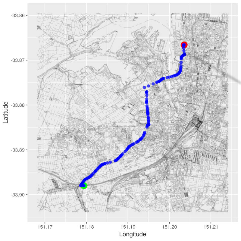
Last time, we learnt about Dijkstra’s algorithm and implemented it in R. We found the shortest path from Newtown Station to Small Bar.
But this is not enough for me! I’m obsessed with learning the details of how things work. Merely implementing Dijkstra’s algorithm would leave me feeling empty.
Let’s prove that Dijkstra’s algorithm works!
Proving the “correctness” of Dijkstra’s algorithm
I’ll be analysing the proof found on page 597 of Cormen et al, Introduction to Algorithms, Second Edition. Excellent book - please get it for yourself!
What are we proving?
To quote directly from page 597 of the book:
Dijkstra’s algorithm, run on a weighted, directed graph \(G = (V, E)\) with non- negative weight function \(w\) and source \(s\), terminates with \(d[u] = \delta(s, u)\) for all vertices \(u \in V\)
What in the above quote do we already understand from our knowledge gained from the earlier posts?
- We know what weighted, directed graphs are from my previous posts.
- We also know that a graph \(G\) is made up of a set of vertices \(V\) and a set of edges \(E\).
- We know what a source node \(s\) is.
Let’s define the stuff that we have not yet encountered:
- We don’t know what a weight function is. It’s simply some mathematical function that takes in the set of edges and maps them to real numbers (the weights). More formally, \(w: E \to \mathbb{R}\). In our case, we want non-negative weights only.
- \(d[u]\) is the distance that Dijkstra’s algorithm has calculated from our source node \(s\) to some vertex \(u\) in our set of vertices \(V\).
- \(\delta(s, u)\) is the actual shortest path distance between our source node \(s\) and some vertex \(u \in V\) in our graph.
Now let’s translate the initial quote!
As we mentioned last time, Dijkstra solves the single source shortest path problem. Let’s assume that we know the true shortest distances from our source node to all other nodes in our graph (including the source node itself). Then, to prove that Dijkstra’s algorithm is “correct”, we need to show that when the algorithm terminates, the distances found by Dijkstra from our source node to all other nodes in our graph (including the source node itself) are equal to the “true” shortest distances.
Good!
How do we prove this? We focus on the ‘while’ loop!
To prove the correctness of Dijkstra, the authors focus on the big while loop in Dijkstra. Here are some key lines from our implementation in GitHub from last time:
while (nodes_left_to_process(vec_of_nodes)) {
    ...
    vec_of_nodes <- remove_min_dist_node(vec_of_nodes, min_dist_node_id)
}
In the book, the authors explicitly maintain a set \(S\) of nodes that
have been processed by Dijkstra. The while loop terminates when this
set \(S = V\) (that is, we have processed all nodes in our graph). In
our implementation, we instead maintained a set of nodes that haven’t
been processed yet (vec_of_nodes). Our loop continues until this set
is empty (i.e. when we have processed all nodes in our graph). I will
state everything the authors’ write in terms of our implementation.
If you’re following along with the book, keep this in mind!
The authors use what is called a loop invariant to prove Dijkstra’s correctness. These proofs are broken down into three phases. From page 18 of the book, those three phases are these:
Initialisation: It is true prior to the first iteration of the loop.
Maintenance: If it is true before an iteration of the loop, it remains true before the next iteration.
Termination: When the loop terminates, the invariant gives us a useful property that helps show that the algorithm is correct.
The initialisation phase is like the base case in an induction proof. The maintenance phase is like the inductive step. The termination phase is something different. Unlike in an induction proof, we don’t continue indefinitely. Our algorithm terminates!
The authors use this specific loop invariant:
At the start of each iteration of the while loop … \(d[v] = \delta(s, v)\) for each vertex … (which we have finished processing.)
Time to ATAAAAACK!
Structure of the proof
Let’s tackle each part!
Initialisation
Initially, we have not processed any vertices. So our invariant is trivially true! We are done with this step.
Maintenance
This is where the bulk of the proof is.
Let’s show that when we are done processing our vertex \(u\), \(d[u] = \delta(s, u)\). We don’t go about this directly. We proceed to show this indirectly via a proof by contradiction. We assume something is true. We start to reason and arrive at some contradiction. This contradiction means that our original assumption cannot be true. Therefore, the opposite must be true!
If this is the first time you’ve seen a proof by contradiction, this might be very confusing. If so, see this nice article.
Let’s do this!
Let’s start with an assumption
This is the assumption that we will make which will later give rise to a contradiction:
There is some vertex \(u\) that we have just finished processing which is the first vertex for which \(d[u] \neq \delta(s, u)\).
If we cast our minds back to last time, Dijkstra begins by first processing our source node, \(s\). We set the distance from our source node to our source node to zero in this little function:
initialise_distances_vector <- function(distances_vector, source_node_id) {
  distances_vector[[source_node_id]] <- 0
  return(distances_vector)
}
Therefore, \(d[s]\) (the distance found by Dijkstra from our source node to our source node) is equal to \(\delta(s, s)\) (the true distance from our source node to our source node). They are the same node, so the distance is clearly zero!
So we have our first observation - this mysterious vertex \(u\) cannot be our source node. That is, \(u \neq s\).
Next, we reason that there must be some path from our source node \(s\)
to our node \(u\). Remember the LARGE_NUMBER constant we defined in
our implementation of Dijkstra?
LARGE_NUMBER <- 999999
We set all distances in our vector of distances to this LARGE_NUMBER
in this function:
create_distances_vec <- function(osm_graph, source_node_id) {
  num_nodes <- vcount(osm_graph)
  distances_vec <- rep(LARGE_NUMBER, num_nodes)
  ...
}
In the book, the authors initialise all distances by setting them to
\(\infty\). They are writing a proof in the abstract world of maths. Our
job is to implement the algorithm in an R program. Our choice to use a
LARGE_NUMBER constant of 999,999 metres for our little map of a part
of Sydney has the same practical effect. However, as we are
mathematically proving the properties of our algorithm, let’s talk in
terms of \(\infty\).
The authors reason that there must be some path from \(s\) to \(u\), because if there was no path at all, \(d[u] = \delta(s, u) = \infty\). That is, the distance found by Dijkstra would remain as the \(\infty\) value we initialised it with, and therefore, our algorithm would have found the “correct” distance from \(s\) to \(u\) (which happens to be \(\infty\) because there is no path in our graph from \(s\) to \(u\)). If our algorithm found the correct distance between \(s\) and \(u\), then this would have violated our initial assumption that \(d[u] \neq \delta(s, u)\).
We are safe to proceed! We have our second observation - there is some path between \(s\) and \(u\). And because there is “some path”, there must exist a shortest path!
To explain the next part, let’s refer to this image which can be found on p597 of the book:
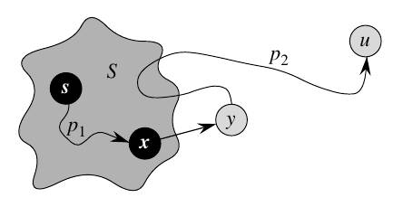
This image shows us some path \(p\), which connects our source node \(s\) to our vertex \(u\). The dark blob named \(S\) is the set of nodes that have already been processed.
We have a vertex \(y\) which is the first vertex along the path \(p\) that has not been processed yet (notice how it is outside of the dark blob \(S\)). \(x\) is the predecessor on this path (i.e. the vertex directly before \(y\)), and has already been processed by our algorithm.
The authors reason that because \(u\) is the first vertex for which our algorithm fails to find the actual shortest path, when \(x\) was processed, Dijkstra must have found the correct shortest path. That is, \(d[x] = \delta(s, x)\). When we processed \(x\), all edges out of \(x\) were relaxed. These are the relevant lines in our implementation:
for (i in seq_along(adjacent_to_min_dist_node)) {
  ...
  if (current_distance_to + distance_to_adj_node < curr_known_dist_to_adj_node) {
    vec_of_distances[[adjacent_node_id]] <- current_distance_to + distance_to_adj_node
    vec_of_predecessors[[adjacent_node_id]] = min_dist_node_id
  }
  ...
}
This means that the algorithm found the correct shortest path distance to \(y\)! That is, we have \(d[y] = \delta(s, y)\).
Let’s contradict our assumption!
We started with an initial assumption that our algorithm found the wrong shortest path distance for our vertex \(u\). That is, \(d[u] \neq \delta(s, u)\). We assumed that \(u\) was the first vertex where this had happened. We will now contradict our assumption and show that in fact \(d[u] = \delta(s, u)\)!
The vertex \(y\) occurs prior to \(u\) on some shortest path. Therefore, the shortest path distance between our source \(s\) and \(y\) must be less than or equal to our distance from our source node to \(u\). Why less than or equal to? Because \(y\) and \(u\) may be the same node. So \(\delta(s, y) \leq \delta(s, u)\). This means that:
\[d[y] = \delta(s, y) \leq \delta(s, u) \leq d[u]\]The last bit \(\delta(s, u) \leq d[u]\) is relevant because Dijkstra relaxes edge
weights downward from our initial LARGE_NUMBER value and continues to
decrease the edge weights until their reach their lower bounds. If
\(\delta(s, u)\) is the lower bound, then the smallest edge weight
\(d[u]\) that the algorithm can find is \(\delta(s, u)\).
The authors then continue - both \(u\) and \(y\) were unprocessed when our algorithm chose \(u\) to process in its while loop. So that means, \(d[u] \leq d[y]\) and that:
\[d[y] = \delta(s, y) = \delta(s, u) = d[u]\]What??? Did you see that???
\[\delta(s, u) = d[u]\]CONTRADICTION!!!
This means that when our algorithm is done processing \(u\), we have in fact found the actual shortest path between our source \(s\) and \(u\) and that this shortest distance is maintained through to when the algorithm terminates.
Hooray! Our maintenance step is complete.
Termination
This step is simple! Once our algorithm terminates, we have finished processing all vertices. That is, our vector of nodes left to process is empty and our loop stops:
while (nodes_left_to_process(vec_of_nodes)) {
  ...
}
This termination phase along with the maintenance phase above show that Dijkstra’s algorithm finds the shortest path distance for all vertices \(u \in V\) (where \(V\) is the set of vertices in our graph).
Next time
Mathematics can be difficult…but I see so much beauty in it! The way the steps in mathematical proofs flow is breathtaking.
Next time, I will finally write about how I came up with different routes to walk to work! It involves a little bit of geometry ;)
Justin