I walk the (train) line - part un
(TL;DR: author begins quest to use undiagnosed OCD to come up with different paths to walk to work…all in the name of weight loss)
I love to walk.
I’m in between jobs. Despite being offered the same rent for another year after concluding my data-driven battle with my real estate agent, I’ve moved apartments. All of this means less time to cook, and more time for fast food. McDonald’s Monopoly is around so how could I resist? I’ve won a Big Mac, a sundae and a small fries so far. What else could I win?
As a result, I’ve put on a bit of weight. So I have started to walk to work a lot. But I find myself getting off the train at Newtown station and walking to the city via the the same route everyday.
I need a way to mix up the routes to work between Newtown and the CBD.
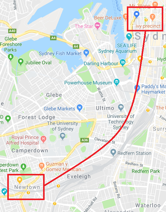
More importantly, I need to feed my tendency to obsess over most things mathematical and technical.
Let’s go on an adventure!
Graphs, maps and almost no maths
A street map can be represented as a graph. When you hear the word ‘graph’, you probably think of some sort of chart. You might even think of the graphs of mathematical functions that you would have encountered in high school:
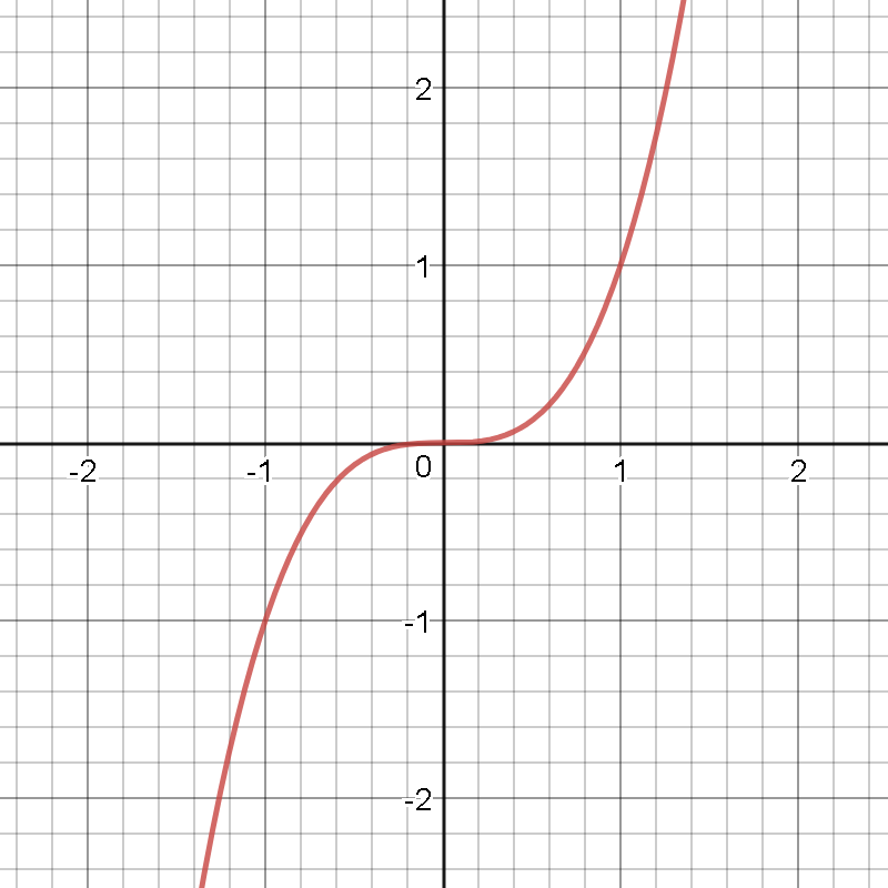
But what I mean by the word ‘graph’ is something like this:
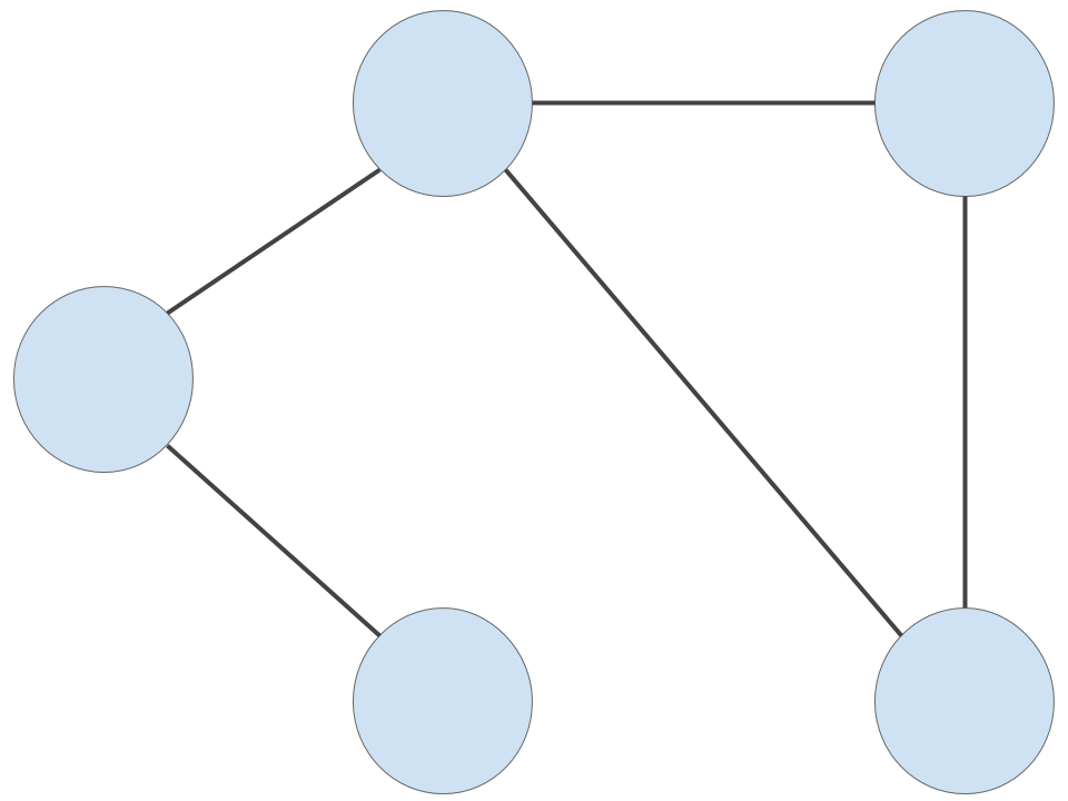
The circles are vertices, and the lines connecting the vertices are edges.
The graph above is an undirected graph - there is no restriction on the direction of travel along any given edge. Here is a directed graph, where there may be restrictions placed on which way we may travel along a given edge:
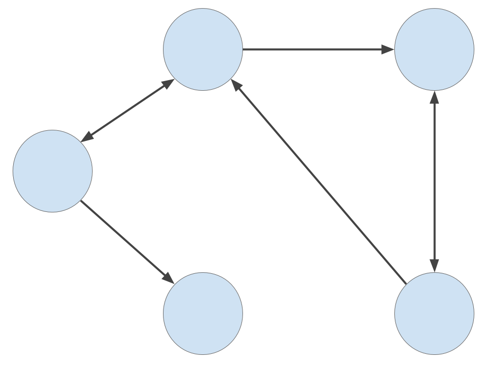
When talking about directed graphs, the circles are often called nodes and the directed edges are often called arcs. But let’s not worry about this distinction. For our purposes, a graph G is a mathematical structure defined as
G = (V, E)
where V is a set of vertices and E is a set of edges. In other words, a graph is a collection of vertices and edges. Not too difficult, right?
What does this have to do with walking to work?
Let’s take a look at a common representation of a street map. This is one of an area in Newtown:
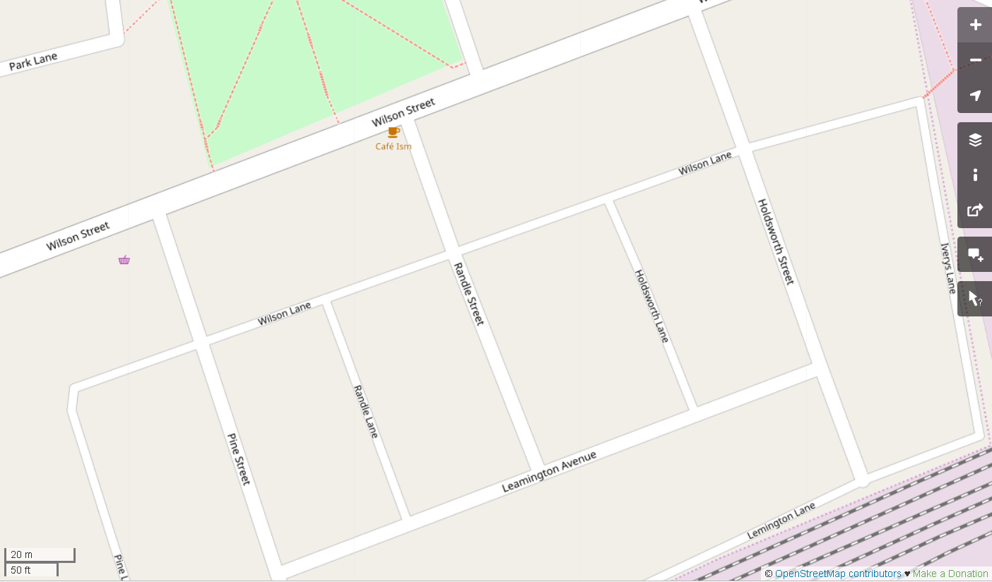
Let’s strip out everything but the basics. This is an abstract representation of the same map:
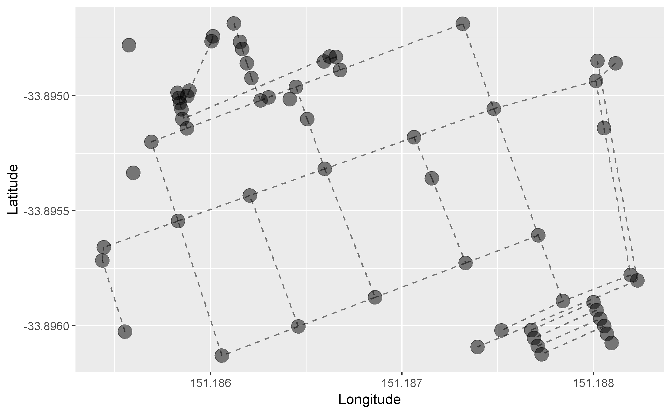
This is a graph! Pretty cool, right?
We can see that each intersection is represented by a vertex. There are also some vertices that don’t appear to be connected by edges. These represent points of interest such as shops.
Where the data at? OpenStreetMap!
I don’t know what I would do without access to open-source data and software. I’m a big fan of the open-source philosophy. In honour of R (which is open-source) and open-source slack emojis, let’s take a minute to dance:

Note: The above works on several levels. The parrot that inspired this amazing Slack emoji is the endangered kakapo from New Zealand. R was created in New Zealand. I’m part kiwi. We’re a bunch of open-source kiwis! For more hilarious party parrot emojis, visit the Cult of the Party Parrot. You won’t be disappointed!
OpenStreetMap
The OpenStreetMap project was founded in 2004 by Steve Coast. Its goal is to promote the development and distribution of open-source geospatial data. Data is contributed to OpenStreetMap by a community of mappers. Click here to find out how to start contributing yourself.
How do I get data out of this thing? Exporting data directly from OpenStreetMap
On the OpenStreetMap website, you can navigate to an area of a map and export the data directly from your browser:
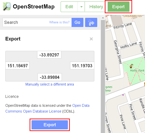
This approach to get map data works well when you’re zoomed in and, as a result, you don’t need to download much map information from the OpenStreetMap API. If you zoom out and try to export a larger area of a map that contains more than 50,000 nodes, you will be presented with an error.
I need to find another source. Remember the coordinates present in the image, above. We’ll use these later.
Download ALL the things (with help from Geofabrik)
The good people at Geofabrik update huge extracts of OpenStreetMap data each evening. The world is carved up into a collection of regions, which may be further split into sub-regions. Even Antarctica makes an appearance.
We’re only interested in Australia so let’s navigate to ‘Australia and Oceania’ under ‘Sub Region’.
Next, we’re presented with a number of different file types. The R package that we’ll use below has a function to read ‘.osm’ files directly into R. However, the ‘.osm’ file for Australia is about 7 gigs when uncompressed. R takes far too long to read this into memory. So we’ll download the ‘.osm.bz2’ file, extract the single file contained within, and subset it outside of R into a smaller, more manageable region. This smaller region will be a map containing the area between Newtown and the CBD only.

Process the data: Osmosis, I choose you
Osmosis is a Java application that is built to process OpenStreetMap data. Specifically, we’re going to use it subset the file containing all of Australia into the area encolsed by this bounding box stated in terms of latitude and longitude in the decimal degrees format:
- left = 151.1681
- bottom = -33.9039
- right = 151.2142
- top = -33.8595
How did I come up with these? And why the need for 4 decimal places of precision? Am I that pedantic? I will answer these questions in reverse order:
- Am I that pedantic? - No.
- Why do I need 4 decimal places of precision? - I don’t.
- How did I come up with these? - Remember when we tried to export map data directly from the OpenStreetMap website? I simply zoomed into an area of the map that contained both Newtown and the CBD, clicked on the ‘Export’ button and voila! Coordinates!
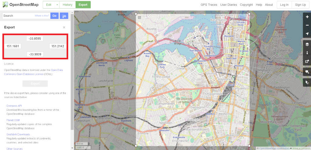
To download Osmosis, click here and follow the instructions. Take note of where your Osmosis ‘bin’ folder is. In my case, it is here:
osmosis_path <- 'C:\\osmosis-latest\\bin'
Note the double backslashes. I’m on a Windows machine where paths are delimited by backslashes. A backslash is a special character in R that means ‘process the character immediately to the right as text’. This is called ‘escaping’. So I need to ‘escape’ the backslash itself with another backslash so that the first backslash is processed as text, and not as the ‘escaping’ character. Sorry about the gratuitous use of the word ‘backslash’.
As this is a Java application, you will need to have the Java Runtime Environment installed on your computer. Install it and take note of the full path to the ‘javapath’ folder. For me, this is where it exists:
java_path <- 'C:\\Program Files (x86)\\Common Files\\Oracle\\Java\\javapath'
We will be using this information…right now!
Set the PATH
The Java folder may already exist in your system PATH variable. Osmosis may also exist in the variable. You can find out by issuing:
Sys.getenv('PATH')
But who cares? Let’s make sure that they are in your PATH variable by putting them there now. If you ran the above line, you will see that the variables are separated by semicolons. So we will make sure to use semicolons to separate our new paths:
Sys.setenv(PATH = paste(Sys.getenv('PATH'), osmosis_path, java_path, sep = ';'))
Subset our OpenStreetMap XML
My normal project workflow is to have ‘input’ and ‘output’ folders located in my working directory. Let’s set up variables pointing to these two folders:
in_dir <- file.path(getwd(), 'input')
out_dir <- file.path(getwd(), 'output')
I have extracted the ‘.osm’ file we downloaded earlier into the ‘input’ folder. Let’s take note of the path to this file.
osm_file_path <- file.path(in_dir, 'australia-latest.osm')
Remember how we added the ‘bin’ directory of Osmosis to our PATH variable? If you open up your terminal and type ‘osmosis’, you will see that it does something:
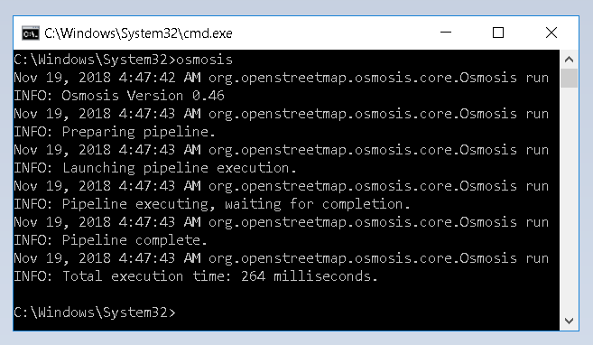
If you don’t see any Osmosis-related info, then you will need to make sure that the ‘bin’ directory of Osmosis is in fact in your PATH variable. Google and Stack Overflow are your friends!
Note: Most of the following Osmosis-related code is based on the vignette contained within the osmar package which will use in this artice soon. I give full credit to those great authors.
We are going to issue a command to the terminal like this one:
osmosis --read-xml file=D:\\blog\\input\\australia-latest.osm enableDateParsing=no
  --bounding-box top=-33.8595 left=151.1681 bottom=-33.9039 right=151.2142
  --write-xml file=C:\\temp\\file2cc826c5214a
This command reads in the ‘.osm’ file we downloaded, subsets it based on some coordinates, and outputs the subset to a temporary location. Once it is output to this temporary location, we will read it into R and we are done with the command line.
We alredy know where our ‘.osm’ file is located, so the input part of the command is sorted. We will now create variables to hold the location of the edges of our bounding box. We came up with these earlier by using the OpenStreetMap website:
left <- 151.1681
bottom <- -33.9039
right <- 151.2142
top <- -33.8595
Next, we create a temporary file to write the subset to. The tempfile() function returns the path to the temporary file we will be creating.
temp_file <- tempfile()
Let’s build the command that we will issue to the terminal.
input_command <- sprintf('--read-xml file=%s', osm_file_path)
args <- sprintf('--bounding-box top=%s left=%s bottom=%s right=%s', top, left, bottom, right)
output_command <- sprintf('--write-xml file=%s', temp_file)
request <- sprintf('osmosis %s %s %s', input_command, args, output_command)
Let’s take a look at what we’ve built.
print(request)
## [1] "osmosis --read-xml file=D:/Desktop/blog/walking_the_train_line_part_un/input/australia-latest.osm --bounding-box top=-33.8595 left=151.1681 bottom=-33.9039 right=151.2142 --write-xml file=C:\\Users\\eustin\\AppData\\Local\\Temp\\RtmpqQhzdO\\file34c02503f71"
Good. Execute!
system('cmd.exe', input = request)
The output should look something like this:
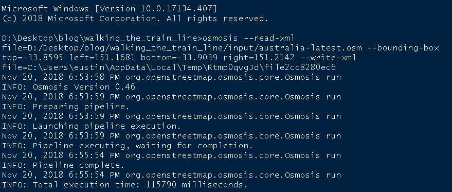
Once Osmosis finishes processing the file, we can read in the subset ‘.osm’ file it created. The file is in OSM XML format and we will use a function provided in the osmar package (introduced next) to convert it into an osmar object.
osm_data <- readLines(temp_file)
osm_data <- as_osmar(xmlParse(osm_data))
Let’s do some housekeeping and remove our temp file.
unlink(temp_file)
For some reason, I get problems with the timestamp field when using the piping operator, so let’s remove that field.
osm_data$nodes$attrs$timestamp <- NULL
osm_data$ways$attrs$timestamp <- NULL
osm_data$relations$attrs$timestamp <- NULL
A little bit about the OpenStreetMap data model
The basic elements that make up the OpenStreetMap data model are nodes, ways and relations. Each one of these can have tags associated with them which provide more information about the elements in question.
Nodes are points on the Earth’s surface defined by their latitudes and longitudes. An example of a node is an intersection. Ways are ordered lists of nodes. An example of a way is a road. Relations describe the relationship between nodes, ways and even other relations. We will not be using them here.
Tags are described in ‘key:value’ format. An example of a tag on a node is ‘name:Australia Post’, where:
key = name
and
value = Australia Post
Enough! Let’s use our data.
Working with the data - osmar
The osmar package allows us to work with OSM XML within the R-universe. It contains functions to convert our osmar objects into graphs which will become important in the second part of this article.
You can easily plot the map contained within our osmar object.
plot_ways(osm_data)
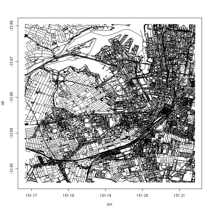
But I’ll be plotting using the pretty_graph() function I wrote…because it’s (slightly) prettier! It also uses ggplot2 which means that the default settings for our visualisations will likely be pretty.
pretty_graph(osm_data)
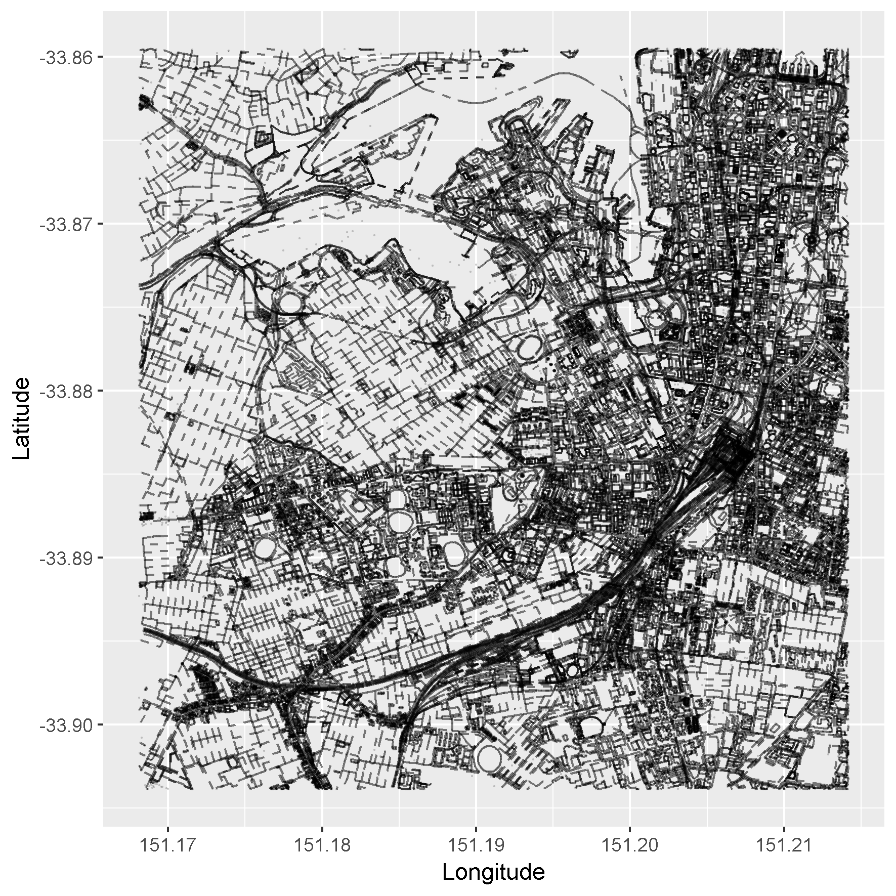
Full code for pretty_graph() is provided at the end of this article.
Find the start and end point of our paths
Back to my original goal - finding paths between Newtown and the CBD. I will show you two ways to find the starting and ending nodes of the paths we want to find on our map.
Export data directly from OpenStreetMap
This is probably the simpler of the two ways I will show you:
- Go to openstreetmap.org
- Navigate to a part of the map that is small enough to export using the ‘Export’ button.
- Open the downloaded ‘map.osm’ file in a text editor.
- Use ‘Find’ in your text editor to find the node ID you’re after.
Here, I searched for the word ‘station’ and located the node ID for Newtown Station:

Use osmar’s find() function
In this tricker (and more fun) version, we will use osmar’s find() function, which is defined as follows:
find(osmar_object, elements_to_extract(where_to_look(conditions)))
In (almost) plain English:
- within our osmar_object,
- find elements_to_extract that meet some conditions applied to data contained within where_to_look, and
- return those elements_to_extract that meet those conditions
elements_to_extract are OpenStreetMap elements such as nodes, ways and relations. where_to_look will normally be the tags associated with nodes, ways and relations. The conditions will normally be something like “where the value in the tag is ‘station’”.
Here is a concrete example. To return all nodes that contain the tag ‘railway:station’, we can issue:
find(osm_data, node(tags(k == 'railway' & v == 'station')))
Applying our description above to this example:
- within our osmar_object,
- find nodes where the key is ‘railway’ and the value is ‘station’ within the tags associated with the nodes, and
- return those nodes that meet the condition in 2, above.
This function returns a vector of node IDs that match the condition we specified:
station_node_ids <- find(osm_data, node(tags(k == 'railway' & v == 'station')))
print(station_node_ids)
##  [1] 1692720118 1763901257 1763901265 1763901272 1763901273 1853704257
##  [7] 1886265379 4735625743 4735626773 5692088717 5692088718 5692088719
## [13] 5692088720 5692089421 5692089422 5692089423 5692089424 5692089425
## [19] 5692089426 5692089427 5692089432 5692089433
But we’re not finished yet. We now have a bunch of node IDs for stations in our map. We’re specifically after the node ID of Newtown Station.
Subsetting osmar objects
We can visually inspect a more manageable subset of our broader osmar object using the subset() function. We’ll use the node IDs we’ve found, above, as an argument to this function.
station_nodes <- subset(osm_data, station_node_ids)
The tags associated with nodes we’ve extracted are conveniently available in data.frame format:
station_nodes$nodes$tags %>%
  head()
##              id         k                                v
## 3111 1692720118      name                    Circular Quay
## 3112 1692720118     layer                                1
## 3113 1692720118   railway                          station
## 3114 1692720118  operator                    Sydney Trains
## 3115 1692720118  wikidata                         Q5121652
## 3116 1692720118 wikipedia en:Circular Quay railway station
By visually (or programatically) looking for the word ‘Newtown’ in the value column (named ‘v’), we find our target! Node ID ‘4735625743’.
rows_to_get <- station_nodes$nodes$tags$v %like% 'Newtown'
newtown_station <- station_nodes$nodes$tags[rows_to_get, 'id']
print(newtown_station)
## [1] 4735625743
Let’s double check by looking at all rows that match our lovely node ID.
rows_to_get <- station_nodes$nodes$tags$id == newtown_station
station_nodes$nodes$tags[rows_to_get, ]
##               id                k       v
## 14938 4735625743             name Newtown
## 14939 4735625743 public_transport station
## 14940 4735625743          railway station
Good…good…
Our terminal node
Let’s just say that I want to lose weight. But I don’t want to lose too much weight. So my terminal node will be Small Bar on Erskine Street (where they do awesome burgers).
Now you give it a go. Try to find that node ID yourself. Assign the node ID of Small Bar to a variable named small_bar.
Wrapping it up (for now)
This article is already pretty dense so I’m going to finish with plotting our map with our start and end nodes highlighted.
Plotting our start and end nodes on our pretty map
First, we will subset our osmar object using our start node ID (newtown_station) and our end node ID (small_bar).
newtown_station <- subset(osm_data, node(newtown_station))
small_bar <- subset(osm_data, node(small_bar))
We use the ‘start’ and ‘end’ arguments of the pretty_graph function to mark our start and end points on top of our map layer.
pretty_graph(osm_data, start = newtown_station, end = small_bar)
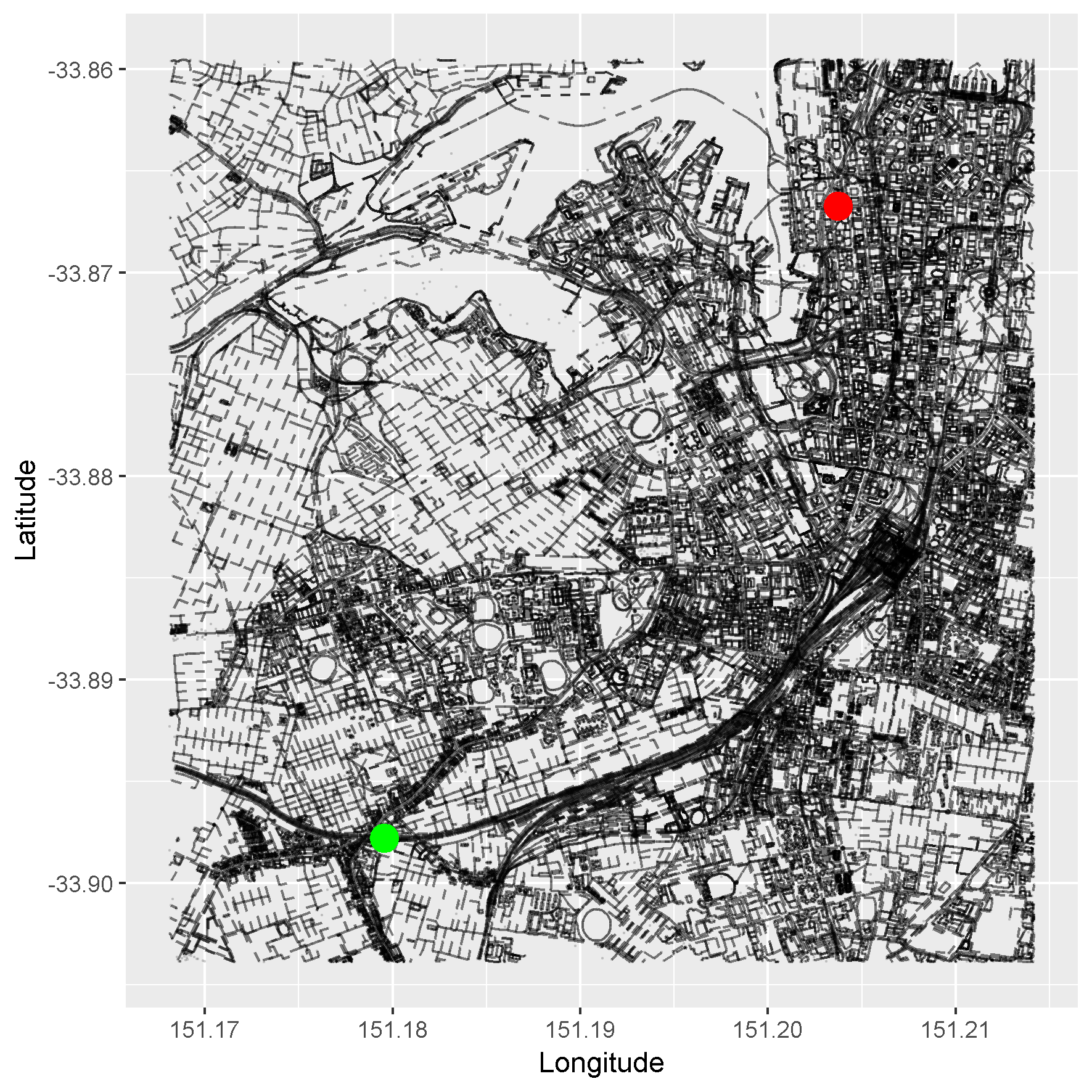
Done!
Next time…
Next time we’ll be doing a little bit of this and completing our quest:
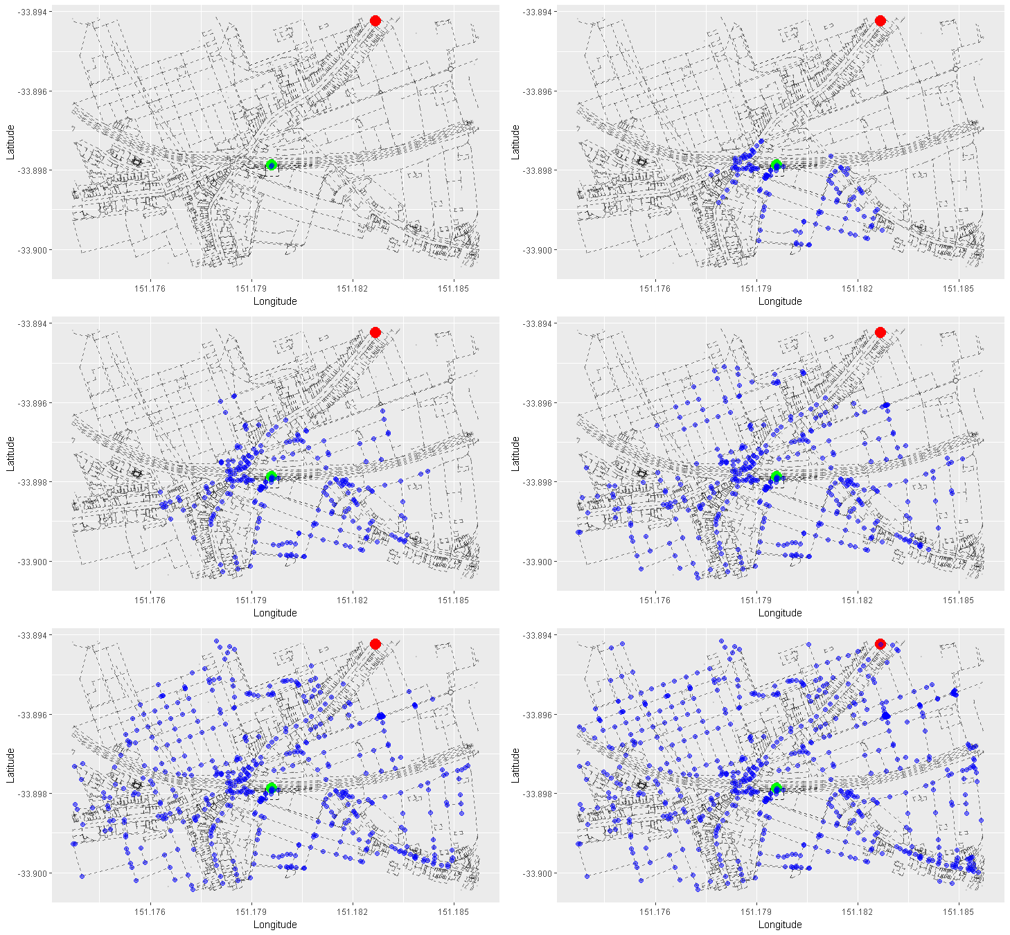
Can you guess what this is showing?
Time to get algorithmic!
Justin
Code
Packages used
The usual arsenal + osmar.
library(ggplot2)
library(dplyr)
library(data.table)
library(osmar)
pretty_graph function
I’ve written some comments in the code below explaining some things. In the above article, we’ve used only used the osm_data, start and end arguments. Here is a description of the arguments we haven’t used:
- path_nodes: We will be using the path_nodes argument next time to plot the paths we find from our start node to our end node.
- path_alpha: This simply controls the opacity of the nodes along the path that we will be plotting.
pretty_graph <- function(osm_data, start = NULL, end = NULL, path_nodes = NULL,
                         path_alpha = 0.5) {
  #
  # input:  osm_data     = an osmar object
  #         start, end   = subset of an osmar object containing the start node
  #                        and end node, respectively
  #         path_nodes   = a character vector of the node IDs we want to plot
  #                        along our path
  #         path_alpha   = the opacity of the nodes along the path we are
  #                        plotting
  #
  # output: ggplot2 plot of our map
  #

  require(ggplot2)
  require(dplyr)

  # extract all node coordinates from our osmar object
  nodes <- osm_data$nodes$attrs
  nodes$timestamp <- NULL
  node_lat <- nodes$lat
  node_lon <- nodes$lon
  node_coords <- data.frame(lat = node_lat, lon = node_lon)

  # if path_nodes provided, extract the coordinates of the
  # nodes along the path we have provided
  if (!is.null(path_nodes)) {
    path_nodes <- find_up(osm_data, node(path_nodes))
    path_nodes <- subset(osm_data, ids = path_nodes)
    path_nodes <- path_nodes$nodes$attrs %>%
      select(lat, lon)
  }

  # we will be plotting all ways and then highlighting a handful of nodes
  # rather than plotting all ways and nodes on the map, which makes the
  # map very 'busy'. taking this approach makes the map look cleaner.
  ways <- osm_data$ways$refs
  ways <- left_join(ways, nodes, by = c('ref' = 'id'))

  # we will be using geom_segment() from ggplot2 so we need to specify the
  # start and end points of each segment. we take the nodes along the ways
  # (which are inherently ordered) and connect them up.
  ways <- ways %>%
    select(ref, id, lat, lon) %>%
    group_by(id) %>%
    mutate(lon_end = lead(lon), lat_end = lead(lat)) %>%
    filter(!is.na(lon_end) & !is.na(lat_end))

  # we start our plotting. our first layer is made up of the ways.
  pretty_plot <- ggplot(node_coords, aes(x = lon, y = lat)) +
    geom_segment(data = ways, aes(x = lon, y = lat, xend = lon_end,
                                  yend = lat_end), linetype = 'dashed',
                 alpha = path_alpha) +
    labs(x = 'Longitude', y = 'Latitude')

  # if the start and/or end nodes have been provided, we layer them next.
  if(!is.null(start)) {
    start <- start$nodes$attrs %>%
      select(lat, lon)
    pretty_plot <- pretty_plot +
      geom_point(data = start, aes(x = lon, y = lat), colour = 'green',
                 size = 5)
  }

  if(!is.null(end)) {
    end <- end$nodes$attrs %>%
      select(lat, lon)
    pretty_plot <- pretty_plot +
      geom_point(data = end, aes(x = lon, y = lat), colour = 'red', size = 5)
  }

  # ...and finally, the path nodes.
  if (!is.null(path_nodes)) {
    pretty_plot <- pretty_plot +
      geom_point(data = path_nodes, aes(x = lon, y = lat), colour = 'blue',
                 size = 2, alpha = path_alpha)
  }

  print(pretty_plot)
}