Learning to rank is good for your ML career - Part 2: let’s implement ListNet!
The second post in an epic to learn to rank lists of things!
Introduction
Now that we know something about word embeddings, let’s use them as inputs into a model that ranks things!
We’ll be working through my implementation of a model called ListNet, which was proposed in this paper:
Cao, Zhe et al. “Learning to rank: from pairwise approach to listwise approach.” ICML ‘07 (2007)
There’ll be a bunch of maths in this post. But don’t worry! We’ll be stepping through it together. I’m here for you!
The setup
Here be our packages for this post.
import random
random.seed(1)

import numpy as np
np.random.seed(1)

import itertools
import matplotlib.pyplot as plt
plt.style.use('ggplot')

import tensorflow as tf
Note: it’s notoriously difficult to make TensorFlow and Keras reproducible. Randomness plays an important part in training neural networks, after all! You might not get the exact numbers shown once we start using TensorFlow later on in the post. But the outcome that I arrive at should be similar to yours! See this post by fellow Aussie Jason Brownlee for more info on this topic.
Let’s start at the end and break it down
Let’s start with a high-level view of what we want to accomplish with ListNet. We’ll use icons of items of clothing in place of our documents because they’re more visually pleasing than article headlines!
We’re going to give ListNet a query, and a bunch of documents to rank. Then, as if through some sorcery, we get a ranked list of documents:
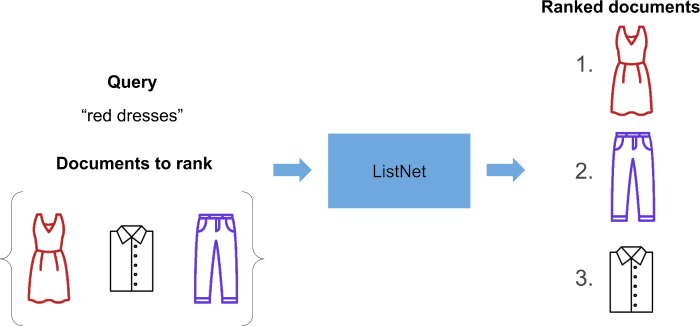
What magic is involved in producing this ranked list? Prepare to be disappointed - ‘cause it ain’t too complex!
ListNet outputs a bunch of real numbers. Each real number is a score assigned to the document we want to rank. We simply sort the documents in descending order of score, and this tells us how the original list of documents should be ranked!
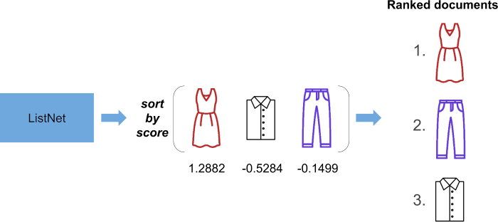
So how does the paper itself describe ListNet? We find this on page four:
We employ a new learning method for optimizing the listwise loss function based on top one probability, with Neural Network as model and Gradient Descent as optimization algorithm. We refer to the method as ListNet.
Let’s break this down and attack it’s smaller pieces relentlessly in our usual way!
We’ll attack in this order:
What do they mean by listwise?
What is this top one probability they speak of?
What is the listwise loss function?
What is the neural network architecture?
If you’ve been reading this, I’ll assume that you know what gradient descent is.
Let’s do this!
What’s a ‘listwise approach’ to learning to rank?
Let’s start with our first question!
There are several approaches to learning to rank. In Li, Hang. (2011). A Short Introduction to Learning to Rank., the author describes three such approaches: pointwise, pairwise and listwise approaches.
On page seven, the author describes listwise approaches:
The listwise approach addresses the ranking problem in a more straightforward way. Specifically, it takes ranking lists as instances in both learning and prediction. The group structure of ranking is maintained and ranking evaluation measures can be more directly incorporated into the loss functions in learning.
Alright! That’s not too bad. We can make some observations at this point.
Firstly, pointwise and pairwise approaches ignore the group structure of rankings. Lists can be thought of as groups of objects placed in specific orders. It makes sense that if we take a listwise approach that the structure of objects within our list is maintained!
Learning to rank often involves optimising a surrogate loss function. This is because the loss function that we want to optimise for our ranking task may be difficult to minimise because it isn’t continuous and uses sorting! ListNet allows us to construct our ranking task in such a way that decreasing its loss values more directly impacts our “true” objective (for example, increasing Normalised Discounted Cumulative Gain or Mean Average Precision).
First question answered. Tick!
Where do probabilities fit into ListNet?
The authors use a probability-based approach to map their lists of scores to probability distributions. Once this is done, they calculate their loss between the predicted probability distribution and a target probability distribution. The authors describe their rationale for defining the problem in this way on page three:
We assume that there is uncertainty in the prediction of ranking lists (permutations) using the ranking function. In other words, any permutation is assumed to be possible, but different permutations may have different likelihood calculated based on the ranking function. We define the permutation probability, so that it has desirable properties for representing the likelihood of a permutation (ranking list), given the ranking function.
Very nice! The two probability models described are the permutation and top one probability models. We’ll now go through them in turn.
Warning: detail ahead!
If you’re pragmatic, then I’ll let you in on a secret: the authors end up using the top one probability model so you can skip the section on ‘permutation probability’.
However, if you have a burning desire to understand things from their deepest depths, read on! Let’s flex our mathematical muscles!
Permutation probability
Let’s use the same ‘dress’, ‘shirt’ and ‘pants’ example from above. We have \(n = 3\) objects to rank:
objects_to_rank = {'dress', 'shirt', 'pants'}

What are all the possible permutations of these three objects?
all_permutations = list(itertools.permutations(objects_to_rank))

for x in sorted(all_permutations):
    print(x)
('dress', 'pants', 'shirt')
('dress', 'shirt', 'pants')
('pants', 'dress', 'shirt')
('pants', 'shirt', 'dress')
('shirt', 'dress', 'pants')
('shirt', 'pants', 'dress')
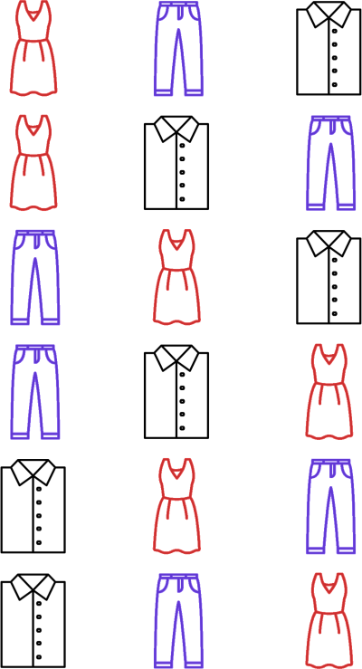
The authors depict this set of possible permutations of \(n\) objects as \(\Omega_n\). The authors depict a single permutation in \(\Omega\) as \(\pi = \langle \pi(1), \pi(2), \dots, \pi(n)\rangle\). Each \(\pi(j)\) denotes the object at position \(j\) in the particular permutation.
Say that each one of these objects is given a real number (a score) by our model which can be used to rank the objects. The authors denote the list of scores associated with each object in a permutation \(\pi\) as \(s = (s_1, s_2, \dots, s_n)\), where each \(s_j\) is the score of the \(j\)-th object.

How can we determine the probability of one of the permutations above, given the ranking function that created these scores?
The authors say that this is how you can do just that:
\[P_s(\pi) = \prod_{j=1}^n \frac{\phi(s_{\pi(j)})}{\sum_{k=j}^n \phi(s_{\pi(k)})}\]This looks like a lot of stuff! But again I say “don’t be scared”! Let’s break it down into tiny pieces.
- Firstly, what are we calculating? We are calculating the probability of some permutation \(\pi\) given some list of scores \(s\). This is depicted by the LHS of the above by \(P_s(\pi)\).
- Next, we notice the big \(\Pi\). This is capital \(\pi\). This symbol says that we will be calculating the product of \(n\) terms. This will become clearer when we go through an example, below.
- Next, we have some \(\phi\)’s. This is the letter ‘phi’. Here, it’s simply some transformation applied to our scores. The only requirement is that it is “an increasing and strictly positive function”, as mentioned on page three.
- The denominator contains a big \(\Sigma\). It tells us that we will be summing \(n - k + 1\) terms. Each one of these terms is a score transformed by the same function \(\phi\).
Walking through an example will clear things up further! We will depict \(\phi\) as an exponential function just like the authors do. Specifically, we will define it as \(\phi(x) = e^x = exp(x)\).
Let’s randomly generate scores for our three objects:
scores_dict = {x: np.random.randn(1)[0] for x in ['shirt', 'pants', 'dress']}

print(scores_dict)
{'dress': 1.6243453636632417, 'shirt': -0.6117564136500754, 'pants': -0.5281717522634557}
Let’s pick one of our permutations:
pi = random.choice(all_permutations)

print(pi)
('dress', 'shirt', 'pants')

obj_pos_1, obj_pos_2, obj_pos_3 = pi

print(f"object at position 1 is '{obj_pos_1}'")
print(f"object at position 2 is '{obj_pos_2}'")
print(f"object at position 3 is '{obj_pos_3}'")
object at position 1 is 'dress'
object at position 2 is 'shirt'
object at position 3 is 'pants'
We get the scores of the objects at the above positions in our permutation:
score_obj_pos_1 = scores_dict[obj_pos_1]
score_obj_pos_2 = scores_dict[obj_pos_2]
score_obj_pos_3 = scores_dict[obj_pos_3]
Let’s write out the \(n = 3\) terms in our product explicitly!
This is what our first term is:
\[\text{first term} = \frac{e^{s_{dress}}}{e^{s_{dress}} + e^{s_{pants}} + e^{s_{shirt}}}\]Evaluating it in Python, we get this:
first_term_numerator = np.exp(score_obj_pos_1)
first_term_denominator = np.exp(score_obj_pos_1) + np.exp(score_obj_pos_2) + np.exp(score_obj_pos_3)

first_term = first_term_numerator / first_term_denominator

print(f"first term is {first_term}")
first term is 0.8176176084739423
According to our formula, this is what our second term is:
\[\text{second term} = \frac{e^{s_{pants}}}{e^{s_{pants}} + e^{s_{shirt}}}\]Evaluating the second term in Python, we get this:
second_term_numerator = np.exp(score_obj_pos_2)
second_term_denominator = np.exp(score_obj_pos_2) + np.exp(score_obj_pos_3)

second_term = second_term_numerator / second_term_denominator

print(f"second term is {second_term}")
second term is 0.47911599189971854
Finally, the third term is this:
\[\text{third term} = \frac{e^{s_{shirt}}}{e^{s_{shirt}}} = 1\]We’ll just assign this value to a variable for the third term:
third_term = 1.0
It’s not that bad when you break it down, right? Putting it all together, the probability of our permutation is then this:
\[P_s(\langle \text{dress, shirt, pants} \rangle) = \prod_{j=1}^3 \frac{e^{s_{\pi(j)}}}{\sum_{k=j}^3 e^{s_{\pi(k)}}}\]This is equivalent to the following:
\[\frac{e^{s_{dress}}}{e^{s_{dress}} + e^{s_{pants}} + e^{s_{shirt}}} \cdot \frac{e^{s_{pants}}}{e^{s_{pants}} + e^{s_{shirt}}} \cdot \frac{e^{s_{shirt}}}{e^{s_{shirt}}}\]Evaluating this in Python, we get this:
prob_of_permutation = first_term * second_term * third_term

print(f"probability of permutation is {prob_of_permutation}")
probability of permutation is 0.39173367147866855
If we calculate the probability of each permutation in our set, we can see that each one is greater than zero and that they sum to one!
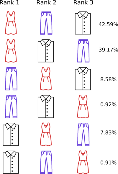
We can make an interesting observation at this point:
The scores sorted in descending order have the highest permutation probability.
The scores sorted in ascending order have the lowest permutation probability.
Interesting! We’re done with the hardest part!
What’s the issue with calculating permutation probability?
To calculate the difference between our distributions using a listwise loss function, we could first calculate the permutation probability distributions for each training example. But this issue with this approach is that there are \(n!\) permutations! The number of permutations that need to be calculated quickly gets out of hand.
Instead, the authors propose using another probability model that is based on “top one” probability.
Top one probability
Given some object we want to rank, \(j\), the top one probability for that object is the sum of the permutation probabilities of the permutations where \(j\) is ranked first.
\[P_s(j) = \sum_{\pi(1)=j,\pi \in \Omega_n} P_s(\pi)\]Given our above example, the top one probability for ‘shirt’ is then \(\approx 0.0783 + 0.0091 = 0.087\).
The authors then observe that to calculate the top one probability of a given object, one doesn’t need to calculate all permutation probabilities of \(n\) objects to rank! The top one probability of our object is equivalent to this:
\[P_s(j) = \frac{exp(s_j)}{\sum_{k=1}^n exp(s_k)}\]where \(s_j\) is the score of the \(j\)-th object.
Let’s not take their word for it…let’s confirm this using Python!
np.exp(scores_dict['shirt']) / sum(np.exp(list(scores_dict.values())))
0.08738232042105001
Would you look at that? It works! The proof of the above can be found in the appendix of the paper for those who are keen.
Converting scores and relevance labels into probability distributions
The astute reader may have realised that the formula we used to calculate our top one probability looks a lot like the softmax function. You are correct! Given the way in which we defined our probability function, We can apply the softmax function to our scores to get the top one probability for each object to rank!
ordered_scores = np.array([scores_dict[x] for x in xlabs]).astype(np.float32)
predicted_prob_dist = tf.nn.softmax(ordered_scores)

print(predicted_prob_dist)
tf.Tensor([0.8176176 0.08738231 0.09500005], shape=(3,), dtype=float32)
Simple! We’ll also convert our relevance grades into probability distributions using the softmax function. We’ll assign each item of clothing an arbitrary relevance grade to illustrate this step:
raw_relevance_grades = tf.constant([3.0, 1.0, 0.0], dtype=tf.float32)
true_prob_dist = tf.nn.softmax(raw_relevance_grades)

print(true_prob_dist)
tf.Tensor([0.8437947 0.11419519 0.04201007], shape=(3,), dtype=float32)
This is what these probability distributions look like:
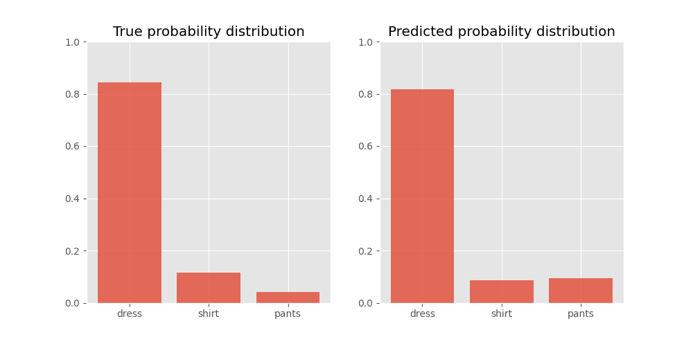
We can see that the score for ‘dress’ ranks it at position one. However, the probabilities for ‘shirt’ and ‘pants’ rank them in the incorrect order.
We now have a probability distribution across our scores and our relevance labels. How can we compare them?
Enter our loss function!
Our loss function - KL divergence
Here’s where we will diverge from the paper. The ListNet paper uses cross entropy as its loss. On page seven, they say this:
Future work includes exploring the performance of other objective function besides cross entropy and the performance of other ranking model instead of linear Neural Network model.
We’ll be using Kullback-Leibler divergence (KL divergence) to explicitly measure the difference between our predicted and target distributions! Let’s learn about it now.
On page seventy-two of ‘Deep Learning’ by Goodfellow et al, the authors describe KL divergence:
If we have two separate probability distributions \(P(X)\) and \(Q(X)\) over the same random variable \(X\), we can measure how different these two distributions are using the Kullback-Leibler (KL) divergence.
Later on the same page, they make this statement:
The KL divergence is \(0\) if and only if \(P\) and \(Q\) are the same distribution in the case of discrete variables.
Given our true and predicted probability distributions, we can define KL divergence in the following way:
\[D_{KL} = \text{true distribution} \cdot \log\left( \frac{\text{true distribution}}{\text{predicted distribution}} \right)\]Let’s apply it to our little clothing example:
sum(true_prob_dist * np.log(true_prob_dist / predicted_prob_dist))
<tf.Tensor: shape=(), dtype=float32, numpy=0.022873338>
This is a small loss value. We see that this makes sense because our true and predicted probability distributions look similar to each other!
We can confirm the second quote from Goodfellow et al by making the following observation:
The logarithm of one is zero. So it follows that KL divergence is zero when both distributions are identical.
Let’s test this out:
sum(true_prob_dist * np.log(true_prob_dist / true_prob_dist))
<tf.Tensor: shape=(), dtype=float32, numpy=0.0>
Hooray! As expected, we get a zero loss when the distributions are identical.
What’s our neural network architecture?
We now know how to transform our document scores into probability distributions. We also know how to compare the probability distribution over our scores to the one over our relevance grades using KL divergence.
We haven’t yet covered how we get our scores in the first place. This is the job of our neural network!
The authors depict a neural network, \(\omega\) and the ranking function based on this neural network as \(f_{\omega}\). The neural network takes in a feature vector \(x_{j}^{(i)}\) and outputs a real number. The feature vector represents a (query, document) pair. You’ll find out how we create these feature vectors later.
We can restate our top one probability equation from above like this:
\[P_{\text{neural net score}}(j) = \frac{exp(\text{neural net score for object }j )}{\sum_{k=1}^n exp(\text{neural net score for object }k)}\]where \(s_j\) is the score of the \(j\)-th object.
We’ve done all the hard work upfront, so this part was easy! Let’s walk through our neural network’s forward pass.
Our inputs
From our first post, we know that we can represent words as embeddings. Let’s use a document retrieval example to illustrate our forward pass. This time, instead of Wikipedia articles, we’ll rank Microsoft Bing and Google search engine results!
Say that we have two queries:
dog
and
what is a dog?
We’ll associate the first query with the top five search results returned by Bing when we perform a search while using that query. We’ll associate the second query with the top five search results returned by Google when we perform a search while using the second query.
query_1 = "dog"

bing_search_results = [
    "Dog - Wikipedia",
    "Adopting a dog or puppy | RSPCA Australia",
    "dog | History, Domestication, Physical Traits, & Breeds",
    "New South Wales | Dogs & Puppies | Gumtree Australia Free",
    "dog - Wiktionary"
]
query_2 = "what is a dog"

google_search_results = [
    "Dog - Wikipedia",
    "Dog - Simple English Wikipedia, the free encyclopedia",
    "Dog | National Geographic",
    "dog | History, Domestication, Physical Traits, & Breeds",
    "What is a Dog | Facts About Dogs | DK Find Out"
]
Let’s assign each document an arbitrary relevance grade:
relevance_grades = tf.constant([
    [3.0, 2.0, 2.0, 2.0, 1.0],
    [3.0, 3.0, 1.0, 1.0, 0.0]
])
At this point, we make an observation:
The number of words in our queries and documents can vary. It follows that the number of word embeddings that make up the queries and documents can vary.
(Note: the number of documents per query can also vary! We’ll deal with how to account for that in the next post, smarty pants!)
How can we remove this variation so that our neural network is given a single feature vector, regardless of how many words are contained in our documents and queries? Let’s answer this question now.
We’ll be using a single embedding matrix for the words in our queries and for our words in our documents. So let’s tokenise our queries and documents using the same Keras Tokenizer:
combined_texts = [query_1, *bing_search_results, query_2, *google_search_results]

tokeniser = tf.keras.preprocessing.text.Tokenizer()
tokeniser.fit_on_texts(combined_texts)

# we add one here to account for the padding word
vocab_size = max(tokeniser.index_word) + 1
print(vocab_size)
35
Here’s our full vocabulary. Notice that there’s no “index 0” as it’s reserved for padding values!
for idx, word in tokeniser.index_word.items():
    print(f"index {idx} - {word}")
index 1 - dog
index 2 - wikipedia
index 3 - a
index 4 - australia
index 5 - history
        ...
        ...
        ...
index 30 - facts
index 31 - about
index 32 - dk
index 33 - find
index 34 - out
Let’s create a bunch of toy embedding vectors. We’ll stick with two-dimensions because we can naturally plot them in our two dimensional plane:
EMBEDDING_DIMS = 2

embeddings = np.random.randn(vocab_size, EMBEDDING_DIMS).astype(np.float32)

print(embeddings)
[[-1.0729686   0.86540765]
 [-2.3015387   1.7448118 ]
 [-0.7612069   0.3190391 ]
 [-0.24937038  1.4621079 ]
 [-2.0601406  -0.3224172 ]
            ...
            ...
            ...
 [-0.29809284  0.48851815]
 [-0.07557172  1.1316293 ]
 [ 1.5198169   2.1855755 ]
 [-1.3964963  -1.4441139 ]
 [-0.5044659   0.16003707]]
Our first query consists of a single word. It can be naturally represented by a single embedding vector:
query_1_embedding_index = tokeniser.texts_to_sequences([query_1])
query_1_embeddings = np.array([embeddings[x] for x in query_1_embedding_index])

print(query_1_embeddings)
[[[-2.3015387 1.7448118]]]
However, our second query consists of four words, so it requires four embeddings to represent it!
query_2_embedding_indices = tokeniser.texts_to_sequences([query_2])
query_2_embeddings = np.array([embeddings[x] for x in query_2_embedding_indices])

print(query_2_embeddings)
[[[-0.93576944 -0.26788807]
  [ 0.53035545 -0.69166076]
  [-0.24937038  1.4621079 ]
  [-2.3015387   1.7448118 ]]]
How can we remove the potential variation in the number of embeddings from query to query and from document to document?
We can aggregate our embedding vectors!
Specifically, we’ll be taking the component-wise average of our word embeddings.
query_2_embeddings_avg = tf.reduce_mean(query_2_embeddings, axis=1, keepdims=True).numpy()

print(query_2_embeddings_avg)
[[[-0.7390808 0.5618427]]]
What does this average vector looked like if we plot it in our two dimensional space?
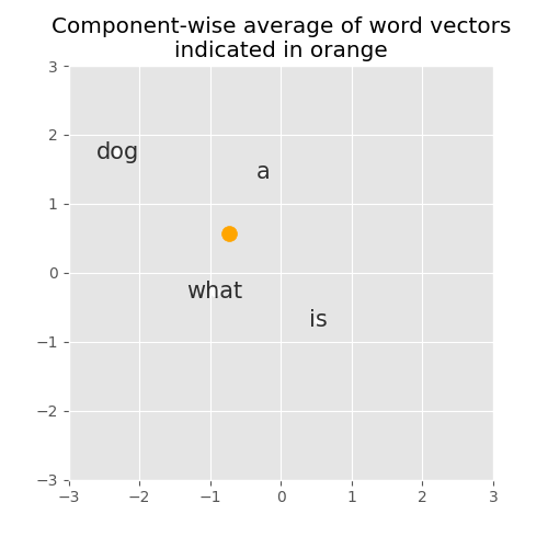
Interesting! This gives us a nice fixed-sized representation of our query.
Let’s create a new array out of the fixed-sized representations of our queries.
query_embeddings = np.row_stack([query_1_embeddings, query_2_embeddings_avg])
Nice! We now have an array of dimensions (number of queries, 1, embedding dimensions), where the “1” represents the number of embedding vectors we have per query after we averaged them. Let’s inspect the shape of our array of queries:
print(query_embeddings.shape)
(2, 1, 2)
Great success! We take the same approach for our documents. We take each word in our document and look up its embedding vector.
docs_sequences = []
for docs_list in [bing_search_results, google_search_results]:
    docs_sequences.append(tokeniser.texts_to_sequences(docs_list))

docs_embeddings = []
for docs_set in docs_sequences:
    this_docs_set = []
    for doc in docs_set:
        this_doc_embeddings = np.array([embeddings[idx] for idx in doc])
        this_docs_set.append(this_doc_embeddings)
    docs_embeddings.append(this_docs_set)
For our Bing results, we get this:
for embeddings in docs_embeddings[0]:
    print()
    print(embeddings)
[[-2.3015387  1.7448118]
 [-0.7612069  0.3190391]]

[[-0.39675352 -0.6871727 ]
 [-0.24937038  1.4621079 ]
 [-2.3015387   1.7448118 ]
 [-0.84520566 -0.6712461 ]
 [-0.0126646  -1.1173104 ]
 [ 0.2344157   1.6598022 ]
 [-2.0601406  -0.3224172 ]]

[[-2.3015387   1.7448118 ]
 [-0.38405436  1.1337694 ]
 [-1.0998913  -0.1724282 ]
 [-0.8778584   0.04221375]
 [ 0.58281523 -1.1006192 ]
 [ 1.1447237   0.9015907 ]]

[[ 0.74204415 -0.19183555]
 [-0.887629   -0.7471583 ]
 [ 1.6924546   0.05080776]
 [ 0.50249434  0.90085596]
 [-0.6369957   0.19091548]
 [ 2.1002553   0.12015896]
 [-2.0601406  -0.3224172 ]
 [-0.68372786 -0.12289023]]

[[-2.3015387   1.7448118 ]
 [ 0.6172031   0.30017033]]
For our Google results, we get this:
for embeddings in docs_embeddings[1]:
    print()
    print(embeddings)
[[-2.3015387  1.7448118]
 [-0.7612069  0.3190391]]

[[-2.3015387   1.7448118 ]
 [-0.35224986 -1.1425182 ]
 [-0.34934273 -0.20889424]
 [-0.7612069   0.3190391 ]
 [ 0.5866232   0.8389834 ]
 [-0.68372786 -0.12289023]
 [ 0.9311021   0.2855873 ]]

[[-2.3015387  1.7448118]
 [ 0.8851412 -0.7543979]
 [ 1.2528682  0.5129298]]

[[-2.3015387   1.7448118 ]
 [-0.38405436  1.1337694 ]
 [-1.0998913  -0.1724282 ]
 [-0.8778584   0.04221375]
 [ 0.58281523 -1.1006192 ]
 [ 1.1447237   0.9015907 ]]

[[-0.93576944 -0.26788807]
 [ 0.53035545 -0.69166076]
 [-0.24937038  1.4621079 ]
 [-2.3015387   1.7448118 ]
 [-0.29809284  0.48851815]
 [-0.07557172  1.1316293 ]
 [ 0.50249434  0.90085596]
 [ 1.5198169   2.1855755 ]
 [-1.3964963  -1.4441139 ]
 [-0.5044659   0.16003707]]
We’ll collapse each document into a fixed-sized vector by averaging them along each of their components. The result is an array with dimensions (number of queries, number of documents per query, embedding dimensions).
docs_averaged_embeddings = []
for docs_set in docs_embeddings:
    this_docs_set = []
    for doc in docs_set:
        this_docs_set.append(tf.reduce_mean(doc, axis=0, keepdims=True))
    concatenated_docs_set = tf.concat(this_docs_set, axis=0).numpy()
    docs_averaged_embeddings.append(concatenated_docs_set)

docs_averaged_embeddings = np.array(docs_averaged_embeddings)
[[[-1.5313728   1.0319254 ]
  [-0.80446535  0.29551077]
  [-0.4893006   0.42488968]
  [ 0.09609441 -0.01519538]
  [-0.8421678   1.0224911 ]]

 [[-1.5313728   1.0319254 ]
  [-0.41862014  0.24487413]
  [-0.0545098   0.50111455]
  [-0.4893006   0.42488968]
  [-0.32086387  0.56698734]]]
We inspect our array’s shape and see that this is so:
print(docs_averaged_embeddings.shape)
(2, 5, 2)
Showing documents in the context of other documents and a query
A single query is potentially associated with multiple documents. Here’s an illustration of our second query with its documents:
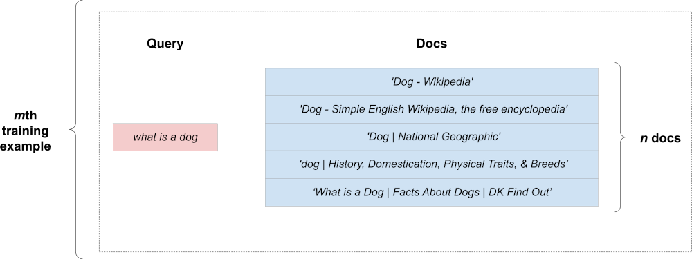
How can we represent a group of documents in the context of a single query? To do this, we can copy the fixed-size representation of our query “n documents times”. We expand our training example into a rectangular shape. Here’s what a single expanded example looks like:
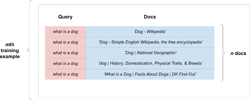
We calculate our loss within the context of each expanded example. We’ll call a batch of such expanded examples as an expanded batch.
How can we repeat our queries as many times as there are documents associated with them using TensorFlow? Thankfully, the TensorFlow ranking repo shows us how we can do this:
NUM_DOCS_PER_QUERY = 5

expanded_queries = tf.gather(query_embeddings, [0 for x in range(NUM_DOCS_PER_QUERY)], axis=1).numpy()

print(expanded_queries)
array([[[-2.3015387,  1.7448118],
        [-2.3015387,  1.7448118],
        [-2.3015387,  1.7448118],
        [-2.3015387,  1.7448118],
        [-2.3015387,  1.7448118]],

       [[-0.7390808,  0.5618427],
        [-0.7390808,  0.5618427],
        [-0.7390808,  0.5618427],
        [-0.7390808,  0.5618427],
        [-0.7390808,  0.5618427]]], dtype=float32)
And to show our groups of documents in the contexts of their associated queries, we simply concatenate them to get our expanded batch:
expanded_batch = np.concatenate([expanded_queries, docs_averaged_embeddings], axis=-1)

print(expanded_batch)
[[[-2.3015387   1.7448118  -1.5313728   1.0319254 ]
  [-2.3015387   1.7448118  -0.80446535  0.29551077]
  [-2.3015387   1.7448118  -0.4893006   0.42488968]
  [-2.3015387   1.7448118   0.09609441 -0.01519538]
  [-2.3015387   1.7448118  -0.8421678   1.0224911 ]]

 [[-0.7390808   0.5618427  -1.5313728   1.0319254 ]
  [-0.7390808   0.5618427  -0.41862014  0.24487413]
  [-0.7390808   0.5618427  -0.0545098   0.50111455]
  [-0.7390808   0.5618427  -0.4893006   0.42488968]
  [-0.7390808   0.5618427  -0.32086387  0.56698734]]]
Not too bad, right?
The hidden layers
We’ll pass our expanded batch into some fully-connected layers. For our prototype, we’ll use a single layer.
Remember what we said about the reproducibility of TensorFlow and Keras results, above!
dense_1 = tf.keras.layers.Dense(units=3, activation='relu')
dense_1_out = dense_1(expanded_batch)

print(dense_1_out)
tf.Tensor(
[[[0.96246356 0.         2.3214347 ]
  [0.5498358  0.         2.0962873 ]
  [0.4715745  0.         2.1984253 ]
  [0.17358822 0.         2.0852127 ]
  [0.72574073 0.         2.414626  ]]

 [[0.8194035  0.         0.91152126]
  [0.26407483 0.         0.7183531 ]
  [0.197609   0.         0.88388896]
  [0.3285144  0.         0.7885119 ]
  [0.30305254 0.         0.87557834]]], shape=(2, 5, 3), dtype=float32)
The output layer - our scores!
This is a dense layer with a single unit. We use a linear unit (i.e. we won’t apply non-linearity to this unit) like in the ListNet paper:
scores = tf.keras.layers.Dense(units=1, activation='linear')
scores_out = scores(dense_1_out)

print(scores_out)
tf.Tensor(
[[[-0.51760715]
  [-0.18927467]
  [-0.10698503]
  [ 0.13695028]
  [-0.29851556]]

 [[-0.58782816]
  [-0.13076714]
  [-0.04999146]
  [-0.1772059 ]
  [-0.14299354]]], shape=(2, 5, 1), dtype=float32)
Calculate KL divergence in the context of our expanded batch
So we now have a bunch of scores. We need to convert them into probability distributions. We observed above that we can do this via the softmax function. So let’s apply it here:
scores_for_softmax = tf.squeeze(scores_out, axis=-1)
scores_prob_dist = tf.nn.softmax(scores_for_softmax, axis=-1)

print(scores_prob_dist)
tf.Tensor(
[[0.14152995 0.19653566 0.21339257 0.27234477 0.17619705]
 [0.1358749  0.21460423 0.23265839 0.20486614 0.21199636]], shape=(2, 5), dtype=float32)
We also observed above that we can do the same for our relevance grades. Let’s apply our softmax function to them here:
relevance_grades_prob_dist = tf.nn.softmax(relevance_grades, axis=-1)

print(relevance_grades_prob_dist)
tf.Tensor(
[[0.44663328 0.1643072  0.1643072  0.1643072  0.06044524]
 [0.4309495  0.4309495  0.05832267 0.05832267 0.02145571]], shape=(2, 5), dtype=float32)
To calculate our batch KL divergence, it’s as simple as doing this:
loss = tf.keras.losses.KLDivergence()
batch_loss = loss(relevance_grades_prob_dist, scores_prob_dist)

print(batch_loss)
tf.Tensor(0.4439875, shape=(), dtype=float32)
But we aren’t satisfied with this simplicity. We must know what this function is calculating behind the scenes!
We already know how to calculate our loss for a single training example:
per_example_loss = tf.reduce_sum(
    relevance_grades_prob_dist * tf.math.log(relevance_grades_prob_dist / scores_prob_dist),
    axis=-1
)

print(per_example_loss)
tf.Tensor([0.29320744 0.5947675 ], shape=(2,), dtype=float32)
To get our batch loss, we’ll simply take the mean of our batch of individual training example losses:
batch_loss = tf.reduce_mean(per_example_loss)

print(batch_loss)
tf.Tensor(0.4439875, shape=(), dtype=float32)
We see the two numbers are the same and have satisfied our yearning for knowledge.
A toy ListNet implemenetation
In the following implementation, we’ll assume a few things. Firstly, I want to leave topics like padding and zero-masking for the next post, so we’ll input our pre-averaged query and document embeddings into our network. Secondly, we’ll be passing our precalculated probability distributions over our relevance grades as only once I’ve covered padding and zero-masking can I show you how to do this dynamically in a training pipeline. Hold your horses for the next post!
We’ll set some constants upfront that depict the dimensions of our data:
NUM_DOCS_PER_QUERY = 5
EMBEDDING_DIMS = 2
We’ll wrap our batch expansion in a custom Keras layer:
class ExpandBatchLayer(tf.keras.layers.Layer):
    def __init__(self, **kwargs):
        super(ExpandBatchLayer, self).__init__(**kwargs)

    def call(self, input):
        queries, docs = input
        batch, num_docs, embedding_dims = tf.unstack(tf.shape(docs))
        expanded_queries = tf.gather(queries, tf.zeros([num_docs], tf.int32), axis=1)
        return tf.concat([expanded_queries, docs], axis=-1)
Once we’ve taken care of the above, the rest of the model is intuitive:
query_input = tf.keras.layers.Input(shape=(1, EMBEDDING_DIMS, ), dtype=tf.float32, name='query')
docs_input = tf.keras.layers.Input(shape=(NUM_DOCS_PER_QUERY, EMBEDDING_DIMS, ), dtype=tf.float32,
                name='docs')

expand_batch = ExpandBatchLayer(name='expand_batch')
dense_1 = tf.keras.layers.Dense(units=3, activation='linear', name='dense_1')
dense_out = tf.keras.layers.Dense(units=1, activation='linear', name='scores')
scores_prob_dist = tf.keras.layers.Dense(units=NUM_DOCS_PER_QUERY, activation='softmax',
                      name='scores_prob_dist')

expanded_batch = expand_batch([query_input, docs_input])
dense_1_out = dense_1(expanded_batch)
scores = tf.keras.layers.Flatten()(dense_out(dense_1_out))
model_out = scores_prob_dist(scores)

model = tf.keras.models.Model(inputs=[query_input, docs_input], outputs=[model_out])

model.compile(optimizer=tf.keras.optimizers.SGD(learning_rate=0.03, momentum=0.9),
              loss=tf.keras.losses.KLDivergence())
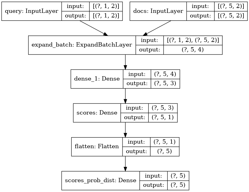
Here be our topology:
Model: "model_1"
__________________________________________________________________________________________________
Layer (type)                    Output Shape         Param #     Connected to
==================================================================================================
query (InputLayer)              [(None, 1, 2)]       0
__________________________________________________________________________________________________
docs (InputLayer)               [(None, 5, 2)]       0
__________________________________________________________________________________________________
expand_batch (ExpandBatchLayer) (None, 5, 4)         0           query[0][0]
                                                                 docs[0][0]
__________________________________________________________________________________________________
dense_1 (Dense)                 (None, 5, 3)         15          expand_batch[0][0]
__________________________________________________________________________________________________
scores (Dense)                  (None, 5, 1)         4           dense_1[0][0]
__________________________________________________________________________________________________
flatten_1 (Flatten)             (None, 5)            0           scores[0][0]
__________________________________________________________________________________________________
scores_prob_dist (Dense)        (None, 5)            30          flatten_1[0][0]
==================================================================================================
Total params: 49
Trainable params: 49
Non-trainable params: 0
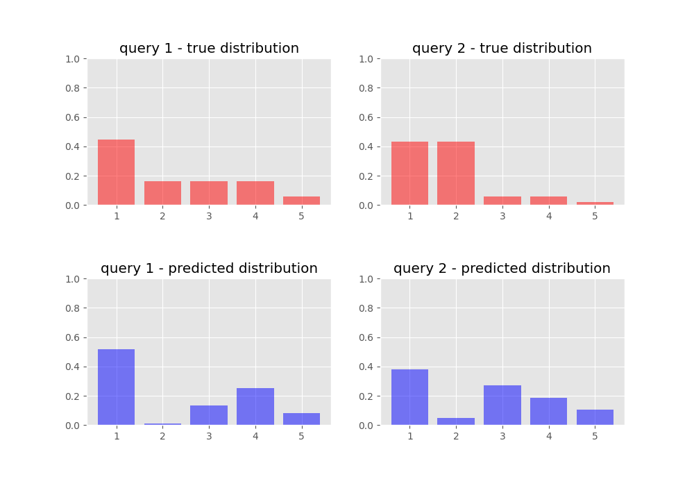
Here’s a comparison of what our target and predicted probability distributions look like before we train our network:
We train for 50 epochs:
hist = model.fit(
    [query_embeddings, docs_averaged_embeddings],
    relevance_grades_prob_dist,
    epochs=50,
    verbose=False
)
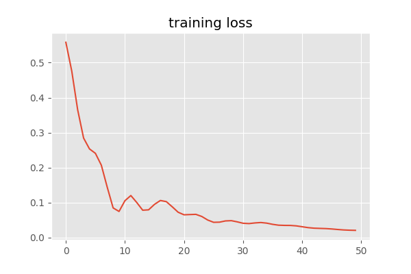
We see that our loss has converged:
We inspect our target and predicted probability distributions once we have trained our network:
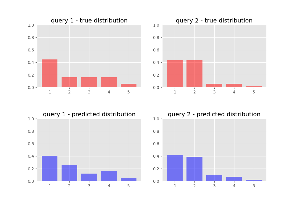
And we jump in joy for our neural network has learnt to rank!
Conclusion
Wow! What an adventure!
We worked through the ListNet paper and we implemented it. Along the way, we covered some of its maths!
Next time, we’ll apply ListNet to a Kaggle competition dataset. We’ll add some stuff to our basic ListNet implementation to cover off some scenarios that come up in real life before we train it on our dataset.
Until next time,
Justin