Learning to rank is good for your ML career - Part 1: background and word embeddings
The first post in an epic to learn to rank lists of things!
A lot of machine learning problems we deal with day to day are classification and regression problems. As a result, we probably have developed some strong intuition on how to approach these types of problems.
But what would we do if we were asked to solve a problem like this one?
Say that each training example in our data set belongs to a customer. Say that we have some feature vector for this customer which serves as an input to our model. For our labels we have an ordered list of products which are ordered by relevance to that customer. How can we go about training a model that learns to rank this list of products in the order described by our labels?
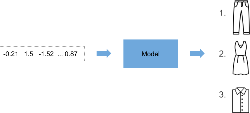
I’ll tell you the tautological answer to this question:
We must ‘learn to rank’!
On this epic
In the first post we’ll be:
- describing a motivating example as an introduction to the field of ‘learning to rank’, and
- exploring word embeddings as we’ll be using them as our features!
In the second post we’ll be:
- learning about the ListNet model architecture, and
- building a prototype of ListNet on some synthetic data.
In the third and final post, we’ll be applying our implementation of ListNet on a Kaggle data set! In that post, we’ll be:
- preparing the above data set so that we can use it with our model,
- training our model, and
- briefly describing Normalised Discounted Cumulative Gain which will serve as our evaluation metric, and
- taking a look at our results!
By the end of this series, I hope that you’ll have some idea of how to approach a similar problem in the future.
What do you mean by ‘learning to rank’?
Much of the following is based on this great paper: Li, Hang. (2011). A Short Introduction to Learning to Rank.
The very first line of this paper summarises the field of ‘learning to rank’:
Learning to rank refers to machine learning techniques for training the model in a ranking task.
Great! That was easy!
The paper then goes on to describe learning to rank in the context of ‘document retrieval’. Let’s use a scenario most of us are familiar with to understand what this is: searching for an article on Wikipedia.
- We have a website, Wikipedia, with a search function.
- Users submit search requests (‘queries’) to the search function.
- Users are then presented with ranked lists of articles (‘documents’).
In learning to rank, the list ranking is performed by a ranking model \(f(q, d)\), where:
- \(f\) is some ranking function that is learnt through supervised learning,
- \(q\) is our query, and
- \(d\) is our document.
Applying this to our Wikipedia example, our user might be looking for an article on ‘dogs’ (the animals). The user types in the word ‘dogs’ into the search bar and is presented with a list of articles that’s ‘sorted by relevance’. The top 3 results are these:
- Dog (redirect from Dogs)
- Dogs Eating Dogs (an EP by the band Blink-182)
- Reservoir Dogs (the Quentin Tarantino film)
This is a well-ranked list for our user!
We mentioned that this is a supervised learning task. What does our training data look like for such a task?
What do our labels look like?
Let’s continue on with our Wikipedia example.
Let’s say that someone has created a dataset by asking real people to submit queries to the Wikipedia search engine and asking them to assign a number to indicate the relevance of an article in the search results set. Let’s say that the curator asks each user to assign each article one of these numbers:
2forrelevant1forsomewhat relevant0forirrelevant
These are arbitrary numbers where the larger the number, the more relevant the article is. We call these relevance grades and are one such way of representing relevance in a learning to rank task.
We should take note of a few things about our example:
- Each query is associated with one or more documents.
- There are as many relevance grades as there are documents associated with a given query.
- We might have multiple articles for a query with the same relevance grade. For example, a user might deem two Wikipedia articles to be ‘somewhat relevant’ to their query. In our example, we are indifferent to the ranking of articles with similar relevance grades. What we will be focusing our efforts on instead is to rank articles with higher relevance grades above those with lower relevance grades.

What features will we be using?
We’ll be using neural nets so we could be using any arbitrary feature that we think might help in our ranking task.
However, for our example, we’ll be focusing on using the words in our queries and documents!
How on earth can we use words as inputs into our neural net? Words aren’t numbers that can be optimised! You’ve lost your mind!
I concede the last statement. But give me a chance to explain. Let’s briefly explore the wonderful world of word embeddings!
Enter word embeddings!
Say that we start with a two-dimensional space:
We’re all familiar with this! Each point in this space can be described by two numbers - an \(x\) coordinate, and a \(y\) coordinate. In other words, each point in the space can be described by pairs of the form \((x, y)\).
Let’s take a word - ‘beagle’. We’ll arbitrarily place it in our space at the point \((2, -1)\):
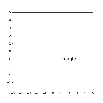
Easy! Now, instead of saying that each point in this space can be described by a ‘pair’, let’s say that it can be described by a ‘vector’. Don’t be scared! Just think of these as lists of numbers! We can depict our vectors like this:
\[\begin{bmatrix} x \\ y\end{bmatrix}\]The first component of our vector represents its coordinate in the first dimension (in this case, the \(x\)-axis), and the second component represents its coordinate in the second dimension (the \(y\)-axis). So taking our beagle example, we can describe our word in this two-dimensional space using this vector:
\[\begin{bmatrix} 2 \\ -1 \end{bmatrix}\]Let’s repeat the process with another word. Let’s plot the name, ‘snoopy’ at the point represented by this vector:
\[\begin{bmatrix}-3 \\ 1 \end{bmatrix}\]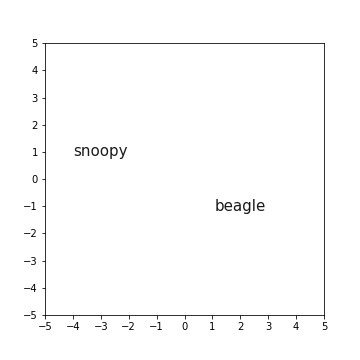
Take a look at that! We have two words which we’ve represented using a bunch of numbers! We call these vectors word embeddings!
A necessary warning
If you’re more pragmatically inclined, then you can stop reading here. Just keep in mind that we’ll be using such word embeddings as our features in the upcoming posts.
However, if you’re more inclined to obsessively understand how things work like I am, then please read on, my friend!
Why would we want to represent our words as embedding vectors?
To understand the benefits of using word embeddings to represent our words, it’s useful to know a bit about how some of the successful language models were built in the past. Let’s go on a journey!
Most of the following summary is based on the ‘12.4 Natural Language Processing’ from the bible of deep learning, ‘Deep Learning’ by Goodfellow et al.
What’s a natural language?
Let’s start with the basics! What’s a natural language? For this, I consult the Wikipedia page for ‘Natural language’:
… a natural language or ordinary language is any language that has evolved naturally in humans through use and repetition without conscious planning or premeditation.
Interesting!
What are tokens?
We need to understand what tokens are to understand what language models are. So, what are ‘tokens’ in the context of natural languages? Say that we have a bunch of sentences. We want to build some model that uses individual words as its smallest units. Then our tokens are individual words. Say that instead, we want to build some model that uses individual characters as its smallest units. Then our tokens are individual characters. Either way, we start with strings and chop them up into useful little pieces. These little pieces are our tokens!
What are language models?
We’re finally ready to define language models. From page 456 of Goodfellow et al:
A language model defines a probability distribution over sequences of tokens in a natural language.
Why would we want to define such probability distributions? Good question! Given our language model, we could ask a question like this:
Which sequence is more likely in our language: “Snoopy is a beagle” or “Beagle Snoopy is”?
If we’ve built our language model using grammatically correct texts, then we would find that the first sequence is more likely to occur than the second one! We could also ask a question like this:
Given the sequence “Snoopy is a”, which word out of my vocabulary of words maximises the probability of the entire sequence?
These probabilities are very useful! For example, they can be used to solve real-life problems like predicting the next word you are about to type in a sentence.
What’s an n-gram?
Many traditional language models are based on specific types of sequences of tokens in a natural language. These are called \(n\)-grams and are simply sequences of \(n\)-tokens! These language models define the conditional probability of the \(n\)-th token given th \(n-1\) tokens that came before it.
You might be wondering:
Why the ‘gram’ in \(n\)-gram?
Apparently it is a Greek suffix which means “something written”!
How were these words represented traditionally?
Traditionally, \(n\)-grams were represented in the one-hot vector space.
Let’s say that we create word-level tokens from our sentence, ‘Snoopy is a beagle’. Let’s create our word tokens from this sentence. At this point, we’ll also import the packages used in this article:
import matplotlib.pyplot as plt
import numpy as np
import tensorflow as tf

sentence = "Snoopy is a beagle"

tokens = sentence.split(" ")

print(tokens)
['Snoopy', 'is', 'a', 'beagle']
We’ll map each word to an index and assign a one to the component at the same index in our one-hot vector. The rest of our components will be zeros.
index_word = {i: x for i, x in enumerate(tokens)}

print(index_word)
{0: 'Snoopy', 1: 'is', 2: 'a', 3: 'beagle'}
num_classes = len(index_word)

index_one_hot = {i: tf.one_hot(x, depth=num_classes) for i, x in enumerate(index_word.keys())}

for k, v in index_one_hot.items():
    word = index_word[k]
    one_hot_vector = v.numpy()
    print(f"{word:<6}: {one_hot_vector}")
Snoopy: [1. 0. 0. 0.]
is    : [0. 1. 0. 0.]
a     : [0. 0. 1. 0.]
beagle: [0. 0. 0. 1.]
We can observe a few things about these vectors.
Firstly, the one-hot vector space is discrete.
Secondly, we can see that the dimensions of our one-hot vectors are as large as our vocabulary is. This is a problem as our vocabulary could consist of millions of words! We can also see that these vectors are sparse (they contain mostly zeros). Embedding vectors on the other hand commonly have dimensions that are far smaller than the sizes of our vocabularies. Each of the components of our embedding vectors are floating-point numbers. They are not sparse but are dense vectors. Given the same number of dimensions, our embedding vectors can represent many more distinct configurations than their one-hot counterparts.
Let’s say that we have our four same words. This time, we’ll represent each word with two-dimensional vectors of floating-point numbers. We’ll randomly create them like this:
embeddings = tf.random.uniform((4, 2), minval=-0.05, maxval=0.05).numpy()

print(embeddings)
[[-0.00841825 -0.02467561]
 [-0.03953496  0.01846253]
 [-0.03010724  0.03095749]
 [-0.01248298  0.00497364]]
Behold the density of these vectors! We’ll come back to these vectors shortly.
Thirdly, we can’t use them to answer questions like “Is the word ‘Snoopy’ more similar to the word ‘beagle’ than it is to the word ‘is’?”. Let’s calculate the Euclidean distance between these vectors. Let’s start with the distance between ‘Snoopy’ and ‘beagle’:
snoopy_vec = index_one_hot[0]
beagle_vec = index_one_hot[3]

snoopy_vs_beagle = tf.sqrt(tf.reduce_sum(tf.square(snoopy_vec - beagle_vec)))

print(snoopy_vs_beagle.numpy())
1.4142135
Next, the distance between ‘Snoopy’ and ‘is’:
is_vec = index_one_hot[1]

snoopy_vs_is = tf.sqrt(tf.reduce_sum(tf.square(snoopy_vec - is_vec)))

print(snoopy_vs_is.numpy())
1.4142135
In both cases, we can see that the distance is \(\sqrt 2\)! These words are equally dissimilar!
Let’s return to our randomly created word vectors. We can see that the distances between these word vectors don’t all equal \(\sqrt 2\)! This is a good start. Assuming that each word vector corresponds to the same words as in the one-hot vector example, we can observe the differences in our Euclidean distances:
snoopy_vs_beagle = tf.sqrt(tf.reduce_sum(tf.square(embeddings[0] - embeddings[3])))

print(snoopy_vs_beagle.numpy())
0.029926574
snoopy_vs_is = tf.sqrt(tf.reduce_sum(tf.square(embeddings[0] - embeddings[1])))

print(snoopy_vs_is.numpy())
0.05318974
Wouldn’t it be nice if we could learn representations for each word where the distance between vectors can be used as a gauge for their similarities?
Let’s now talk about why these dense vectors can help us achieve this. I can’t explain this as well as Yoav Goldberg did in A Primer on Neural Network Models for Natural Language Processing, so I will quote from it!
The author starts with this, beginning on page 6:
The main benefit of the dense representations is in generalization power: if we believe some features may provide similar clues, it is worthwhile to provide a representation that is able to capture these similarities.
The author then describes a scenario:
For example, assume we have observed the word ‘dog’ many times during training, but only observed the word ‘cat’ a handful of times, or not at all.
He then explains what the outcome of this scenario would be if we were to represent the words in the one-hot vector space:
If each of the words is associated with its own dimension, occurrences of ‘dog’ will not tell us anything about the occurrences of ‘cat’.
He then explains what the outcome could be if we were to use word embeddings to represent the same words:
However, in the dense vectors representation the learned vector for ‘dog’ may be similar to the learned vector from ‘cat’, allowing the model to share statistical strength between the two events.
By allowing a concept of a ‘dog’ to be distributed across potentially multiple vectors and multiple dimensions, our dense word embeddings allow us to “recognize that two words are similar without losing the ability to encode each word as distinct from the other” (Goodfellow et al, pages 458-459).
To summarise this section, we can say that word embeddings are generally more efficient and meaningful representations of our words compared to one-hot vectors. We’ll be using these word embeddings as features in the rest of our tutorial.
Let’s build a toy model
Let’s create some ‘sentences’. Each sentence contains two words that share similar meanings.
sentences = [
    "snoopy dog",
    "milo dog",
    "dumbo elephant",
    "portugal country",
    "brazil country",
]
We will represent each of these as word vectors. Our goal is to train a model that places word vectors with similar meanings closer together in some two-dimensional space.
Instead of manually preparing our tokens and assigning indices to them, we’ll use the Keras Tokenizer. Firstly, we’ll create our vocabulary:
tokeniser = tf.keras.preprocessing.text.Tokenizer()
tokeniser.fit_on_texts(sentences)

print(tokeniser.word_index)
{'dog': 1, 'country': 2, 'snoopy': 3, 'milo': 4, 'dumbo': 5, 'elephant': 6, 'portugal': 7, 'brazil': 8}
Then we’ll convert our sentences into sequences of indices which map to words in our vocabulary:
sequences = tokeniser.texts_to_sequences(sentences)
for x in sequences:
    print(x)
[3, 1]
[4, 1]
[5, 6]
[7, 2]
[8, 2]
We take note of the size of our vocabulary which we will use when creating our Embedding layer. Index zero is a special padding value in the Keras Embedding layer so we add one to our largest word index to account for it:
VOCAB_SIZE = max(tokeniser.index_word) + 1
print(f"VOCAB_SIZE: {VOCAB_SIZE}")
VOCAB_SIZE: 9
We want our neural network to learn to pull words in each of our sentences closer together, while also learning to push each word away from a randomly chosen negative example. This negative sampling is accomplished by the negative_samples argument in tf.keras.preprocessing.sequence.skipgrams. We use this function to create a newly sampled training set at the beginning of each epoch:
def make_skipgrams():
    train_x, all_labels = [], []
    for sequence in sequences:
        pairs, labels = tf.keras.preprocessing.sequence.skipgrams(
            sequence, VOCAB_SIZE, negative_samples=1.0, window_size=1, shuffle=True
        )
        train_x.extend(pairs)
        all_labels.extend(labels)

    train_x = np.array(train_x)
    all_labels = np.array(all_labels, dtype=np.float32)

    content_words = train_x[:, 0]
    context_words = train_x[:, 1]

    return content_words, context_words, all_labels
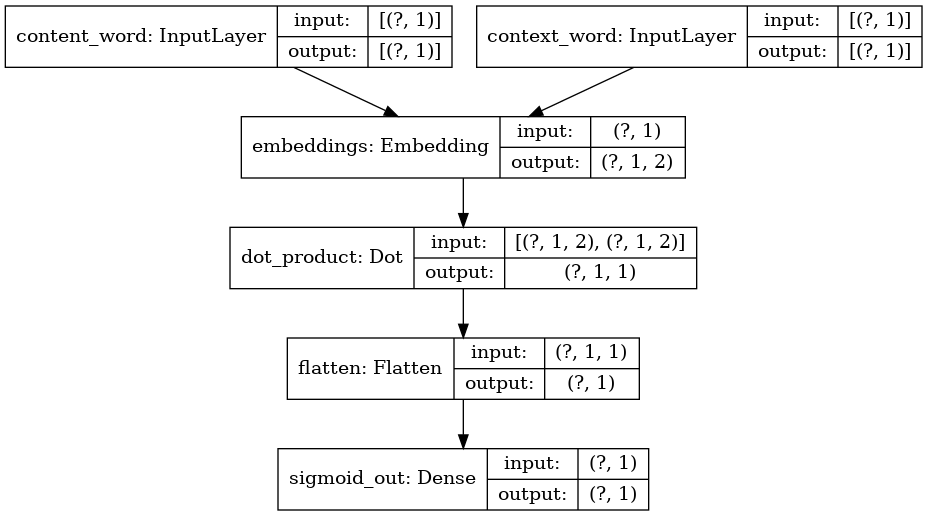
We then build our model. The focus of this post isn’t to explain this toy model so I’ll be brief:
- We input into our network a pair of integers corresponding to the position of our word embedding in our embedding matrix.
- A binary label is passed into the network as well. This label is zero if the two words should be treated as negative examples and it is one if the two words should be associated with each other.
- We look up the corresponding word vectors in our matrix of embedding vectors.
- We calculate the cosine similarity between the two vectors and pass it into our sigmoid unit. This allows us to treat this as a binary classification problem.
# inputs
content_input = tf.keras.layers.Input(shape=(1, ), dtype=tf.int32, name='content_word')
context_input = tf.keras.layers.Input(shape=(1, ), dtype=tf.int32, name='context_word')

# layers
embeddings = tf.keras.layers.Embedding(input_dim=VOCAB_SIZE, output_dim=2, name='embeddings')
dot_prod = tf.keras.layers.Dot(axes=2, normalize=True, name='dot_product')
# graph
content_embedding = embeddings(content_input)
context_embedding = embeddings(context_input)

cosine_sim = tf.keras.layers.Flatten(name='flatten')(dot_prod([content_embedding, context_embedding]))
dense_out = tf.keras.layers.Dense(1, activation='sigmoid', name='sigmoid_out')(cosine_sim)

# model
model = tf.keras.models.Model(inputs=[content_input, context_input], outputs=[dense_out])

DECAY_RATE = 5e-6
LR = 0.1

optimiser = tf.keras.optimizers.SGD(learning_rate=LR, decay=DECAY_RATE)
model.compile(loss='binary_crossentropy', optimizer=optimiser, metrics=['accuracy'])
This is what the above model looks like:
We train the model like this while saving plots of our embedding vectors upon completion of each epoch:
loss_hist = []

for i in range(20):

    if i > 0:

        content_words, context_words, labels = make_skipgrams()

        hist = model.fit([content_words, context_words], labels, epochs=1, verbose=0)
        print(f"loss: {hist.history['loss'][-1]:.4f}")
        loss_hist.extend(hist.history['loss'])

    embedding_vectors = np.array(embeddings.weights[0].numpy())

    fig, ax = plt.subplots(figsize=(10,10))

    ax.scatter(embedding_vectors[1:, 0], embedding_vectors[1:, 1],  c='white')

    for idx, word in sorted(tokeniser.index_word.items()):
        x_coord = embedding_vectors[idx, 0]
        y_coord = embedding_vectors[idx, 1]

        ax.annotate(
            word,
            (x_coord, y_coord),
            horizontalalignment='center',
            verticalalignment='center',
            size=20,
            alpha=0.7
        )

        ax.set_title(f"iteration-{i+1}")

    plt.savefig(f"iteration-{i+1:03d}.jpg")
The result is a bunch of embeddings that move through space!
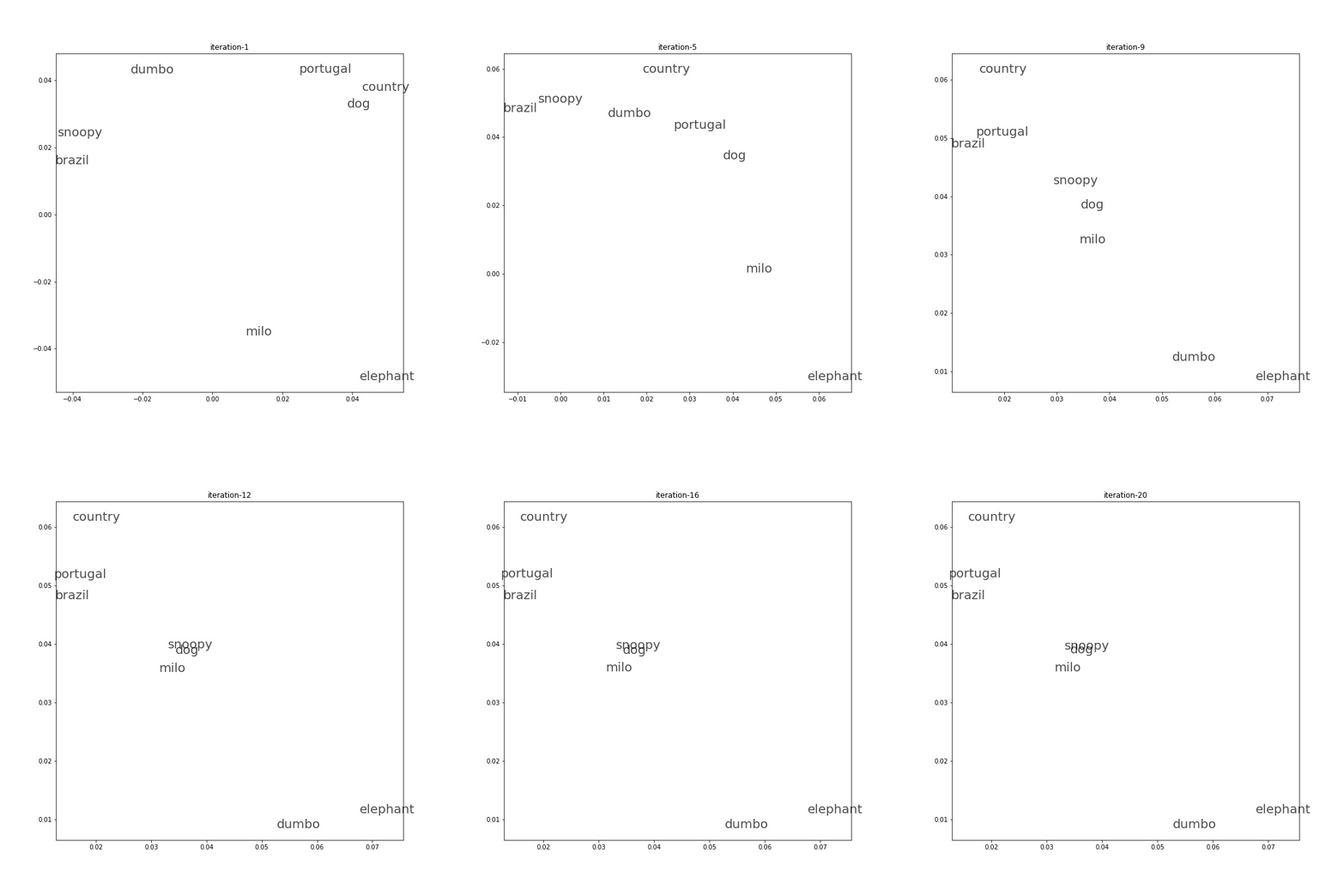
We start out with our words scattered randomly throughout our two-dimensional space. Over the course of twenty epochs, our model has learnt to place the words in our pairs closer together!
Conclusion
We’ve begun our ‘learning to rank’ adventure. We briefly explored a motivating example. We then spent some time exploring word embeddings so that we can use the words in our queries and documents as features in our upcoming model.
Next time, we will be exploring ListNet and implementing it.
Let’s do this!
Justin