Rent-scraping: How I saved money using R
(TD;DR: Received letter from real estate increasing my weekly rent. Reason for increase was not supported by evidence. Used R to look for evidence supporting real estate’s claim. Fought the power.)
Gather ‘round, gather ‘round. Come hear a story of one man’s triumph against the establishment. Read in disbelief as he goes to great lengths to avoid paying a $5 per week rent increase on the grounds that it could not justified by empirical evidence.
(On a serious note: this is about webscraping in R)
“…based on the current market conditions…”
The 12 month lease for my current apartment was coming to an end. Just when I was wondering when the annual email from my real estate agent offering me a new 12 month lease was going to arrive, I received this:
You are currently leasing your property for $500.00 per week and the lease is due to expire on the 18/11/2017. We have recently completed a rental review for your property and advised the owner that based on current market conditions, the rent for your property should increase by $5 per week.
Craving specificity, my mind goes into overdrive: What market conditions? How have they defined them? $5 is so little - what change in market conditions could justify a $5 per week increase?
Having had my rent increased by $20 per week a year ago, a further $5 increase didn’t seem to make sense to me. I also perceived a power imbalance which I didn’t like. On the one hand, we have the real estate agent, who has access to databases of property prices and reports. On the other hand, we have the tennant who does not have access to the same amount of information. This information asymmetry would have traditionally put the tennant in a weaker position and thus more likely to accept the advice of the real estate agent.
Unfortunately for my real estate agent, I’m a little bit crazy.
Where the data at?
I live in a two bedroom apartment with a car space and a single bathroom. I wanted to look for data on apartments with a similar configuration.
NSW Government’s Family & Community Services - “Rent Tables”
I knew that the NSW Government publishes reports on newly rented out houses and apartments on a quarterly basis. There’s a tab in report that shows the first quartile, median and third quartile of the distribution of weekly rent paid for one and two bedroom apartments.
This, of course, isn’t precise enough for me. I know that my rent would more than likely be cheaper if I had no car space. I also know that my rent would be more expensive if I had two bathrooms. So I continue my quest.
Gimme some’in’ to scrape
After some Googling, I found AuHousePrices. Take a look at this screenshot:
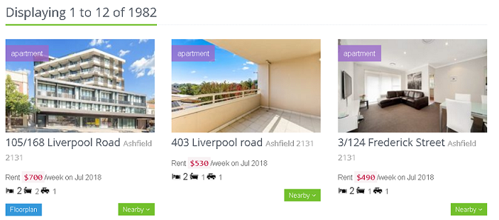
It has all the info that I need:
- the weekly rent,
- the month in which the apartment was leased
- the apartment configuration in terms of the number of bedrooms, bathrooms and car spaces
Another attractive quality of this site was the loop-friendly URL. This is the URL for the first page:
https://www.auhouseprices.com/rent/list/NSW/2131/Ashfield/1/?sort=date&type=apartment&bmin=2&bmax=2
Here is the URL for the second page:
https://www.auhouseprices.com/rent/list/NSW/2131/Ashfield/2/?sort=date&type=apartment&bmin=2&bmax=2
What has changed?
The number after “Ashfield/”!
Now guess what the first 50 URLs might be. Easy, right?
All hail Hadley: R’s rvest package
rvest is a web scraping R package by R royalty, Hadley Wickham. Like most of Hadley’s packages, rvest is simple to use with its intuitive syntax. The package is built to work with the piping operator from magrittr (which users of the dplyr will be familar with), allowing us to create elegant data munging pipelines.
Getting started with rvest is easy:
- Find a page you want to scrape
- Get that page’s url
- Read that page into R using rvest’s read_html() function
- Access the CSS selector containing the data you want using either the html_node() or html_nodes() functions (more on finding the relevant selector and the difference between the functions, below).
- Access the text contained within the CSS selector(s) extracted in the prior step using the html_text() function.
- Use regex to extract relevant text within the CSS selector text accessed in the prior step.
How can we find out which CSS selector contains the data we’re after?
CSS selectors with SelectorGadget
SelectorGadget is a Google Chrome extension that allows you to quickly discover which CSS selector contains the data you’re targeting by simply clicking on it. You no longer have to dig through HTML in your browser’s developer tools. It’s a huge time saver.
Install it…now!
Let’s get-a-scrapin’
We now have all the ingredients necessary to scrape data from websites using R. The output that I ultimately want to create is a time series of weekly rent per the months in which the apartments were leased. I want to make sure that my scraping is working as intended so I want to extract the addresses of the apartments so that I can visually inspect my data against a sample of webpages in Chrome.
Let’s build a prototype and scrape the first page.
library(rvest)
first_page <- read_html('https://www.auhouseprices.com/rent/list/NSW/2131/Ashfield/1/?sort=date&type=apartment&bmin=2&bmax=2')
Target: the addresses
Go into Chrome, and click on the SelectorGadget icon in the top right hand corner. Click on one of the addresses, and you should see something like this pop up in the bottom right hand corner of your browser.
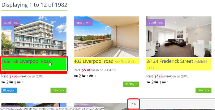
This is the CSS selector that contains the address data. To access the data contained within this selector, we can pipe the page into html_nodes(), specifying the CSS selector name as its argument. To access the text contained within, we can pipe this result into html_text().
Let’s take a look at its output:
first_page %>%
  html_nodes('h4') %>%
  html_text()
##  [1] "2/93 Alt Street Ashfield 2131"
##  [2] "9/23 Orpington Street Ashfield 2131"
##  [3] "9/60 Bland Street Ashfield 2131"
##  [4] "4/122 Frederick Street Ashfield 2131"
##  [5] "3/13 Frederick Street Ashfield 2131"
##  [6] "Address available on request Ashfield 2131"
##  [7] "19/12 Webbs Avenue Ashfield 2131"
##  [8] "132 Frederick Street Ashfield 2131"
##  [9] "17/106 Elizabeth Street Ashfield 2131"
## [10] "106/168 Liverpool Road Ashfield 2131"
## [11] "401/11-13 Hercules Street Ashfield 2131"
## [12] "105/168 Liverpool Road Ashfield 2131"
## [13] " Search Filter and Sorting "
We don’t want element 13 (“ Search Filter and Sorting “) in our vector of addresses, so let’s exclude it.
addresses <- first_page %>%
  html_nodes('h4') %>%
  html_text() %>%
  .[which(. != ' Search Filter and Sorting ')]
Target: the rent per week and month leased
Clicking on the weekly rent and the month in which the apartments were leased presents us with a challenge. The selector that contains the data we’re after (“li”) is shared by a whole bunch of other data. Take a look at the stuff that is highlighted:
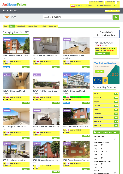
Let’s take a look at the first few elements of what we can extract from the “li” selector:
first_page %>%
  html_nodes('li') %>%
  html_text() %>%
  head(10)
##  [1] "  View By State Melbourne, VIC Sydney, NSW Brisbane, QLD Adelaide, SA Perth, WA Canberra, ACT Darwin, NT Hobart, TAS "
##  [2] "Melbourne, VIC"
##  [3] "Sydney, NSW"
##  [4] "Brisbane, QLD"
##  [5] "Adelaide, SA"
##  [6] "Perth, WA"
##  [7] "Canberra, ACT"
##  [8] "Darwin, NT"
##  [9] "Hobart, TAS"
## [10] ""
We know the pattern of text we want to extract. It goes something like this:
Rent $###/week on Mmm yyyy
Let’s use some regex and the str_extract() function from the stringr package (all Hail Hadley, again) to extract any text matching this pattern in our vector of elements in the “li” selector. Note that str_extract() returns a vector of the same length as the input with NAs for the elements that didn’t match our pattern. We we will filter out the NAs as a final step.
What are all those symbols? A regex to English translation
My claim is that the above pattern can be expressed in regex like this:
^Rent.+/week.*\\d{4}$
Don’t be afraid. It looks crazy, but all this is saying is this:
- ^ - we should match what follows from the beginning of the target string.
- Rent.+ - look for the word “Rent” followed by one or more of any character. The period is a special character in regex which means “match any character”. The plus sign means “one or more” of whatever immediately preceeded it.
- /week.* - look for “per week”, followed by zero or more of any character. The zero or more is expressed using the asterisk, which is the less-strict cousin of the plus sign.
- \\d{4} - the target string should end with 4 digits. “” is another special character in regex which means “match any digit from 0 to 9”. The extra slash is there because we need to escape the backslash in R. “{4}” means “repeat what came immediately before 4 times”. In other words, match 4 digits.
- $ - the target string should end with what came immediately before me. In this case, 4 digits.
Let’s test it out:
library(stringr)

price_month <- first_page %>%
  html_nodes('li') %>%
  html_text() %>%
  str_extract('^Rent.+/week.*\\d{4}$') %>%
  .[which(!is.na(.))]

price_month
##  [1] "Rent $420/week on Aug 2018" "Rent $510/week on Aug 2018"
##  [3] "Rent $490/week on Aug 2018" "Rent $500/week on Aug 2018"
##  [5] "Rent $550/week on Aug 2018" "Rent $730/week on Aug 2018"
##  [7] "Rent $510/week on Jul 2018" "Rent $480/week on Jul 2018"
##  [9] "Rent $520/week on Jul 2018" "Rent $630/week on Jul 2018"
## [11] "Rent $630/week on Jul 2018" "Rent $700/week on Jul 2018"
Woohoo! We have 12 sets of data for the 12 addresses. We can easily break this string apart using more regex to extract the month and the rent per week. I’ll show you how I did it, but try to break it down like I did above and all those symbols will appear less daunting. Firstly, extracting the month…
str_extract(price_month, '[A-Z][a-z]{2} \\d{4}$') %>%
  head(5)
## [1] "Aug 2018" "Aug 2018" "Aug 2018" "Aug 2018" "Aug 2018"
…and then the rent per week:
str_extract(price_month, '(?<=Rent \\$).*(?=/week)') %>%
  head(5)
## [1] "420" "510" "490" "500" "550"
Target: the property configuration
We set out wanting to analyse apartments similar to mine. That is, we want to analyse apartments with 2 bedrooms, 1 bathroom and 1 car space. A look at the search results reveals to us that we need to cater for 2 scenarios:
- most properties have at least one bathroom and at least one car space, so we will have 3 numbers - number of bedrooms, number of bathrooms, and number of car spaces.
- some properties don’t have a car space. So we will have 2 numbers - number of bedrooms, followed by number of bathrooms.
I want to capture both patterns so that I have 12 sets of apartment configurations that they can be easily combined with the sets of 12 addresses, months and weekly rent amounts. Once they have been combined into a data frame, I can easily filter out those apartments that don’t meet my target apartment configuration.
Try translating the below regex into plain English:
first_page %>%
  html_nodes('li') %>%
  html_text() %>%
  str_extract(' \\d \\d (\\d )*$') %>%
  str_trim() %>%
  .[which(!is.na(.))]
##  [1] "2 1 1" "2 1 1" "2 1 1" "2 1 1" "2 1 1" "2 2 1" "2 1 1" "2 1 1"
##  [9] "2 2 1" "2 2 1" "2 2 1" "2 2 1"
Form like Voltron: creating our final dataset
So, what have we learnt?
- We know what the urls for the first n pages are.
- We know how to extract the data of interest on any of these n pages.
All we need to do before we can analyse our data is to write a loop that loops through n pages of apartments while appending each page’s data onto some master dataset. We will then subset this master dataset for apartments that match our desired apartment configuration. Describing this this process is not the focus of this article so I will simply provide my final code at the end of this article.
Dear real estate agent…
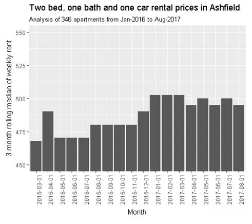
Weekly rent for 2 bedroom, 1 bathroom and 1 car space apartments varied significantly within months.
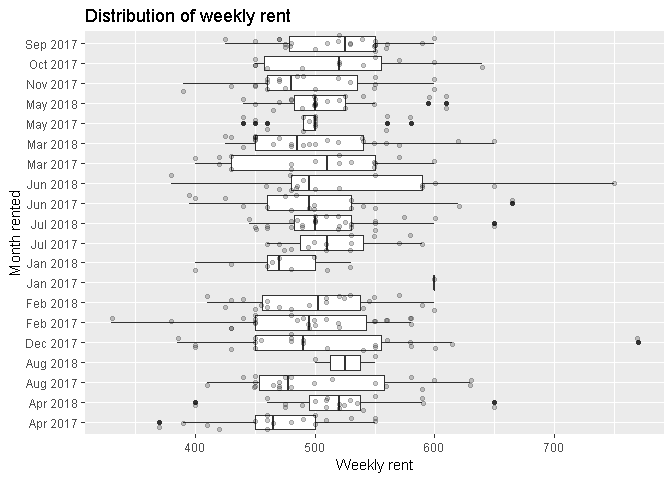
Some possible reasons for what is driving this are these:
- Newer apartments cost more than older apartments to rent - a quick look at the photos of some of the more expensive apartments revealed that they were located in newly constructed apartments right near the train station.
- Apartments closer to the train station and shopping district are more expensive to rent than those that are further away from these.
My apartment is quite old, and about 10 minutes away from the train station. It is by no means exceptional so I felt that a “typical” price would best describe my apartment’s “true” weekly rent. So I played around with some smoothing methods.
I personally love using LOESS via ggplot’s geom_smooth().
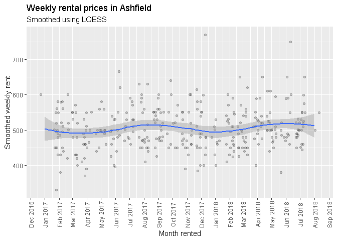
However, I didn’t want to have to explain to my real estate agent how LOESS works. So I settled on a quarterly median rental price. Not as simple as simple as taking an average. But I thought the median was appropriate given the outliers and that it would be easy to explain if I were questioned about my choice of statistic.

So I put this into email:
Rent was increased last year by $20 per week and this appears to be in excess of the market rate at the time (more on this below).
I have performed a review of the data myself and have found that the current rent we pay is fair:
I have used webscraping to collect data on 346 newly rented “two bedroom, one bathroom, one car space” apartments in Ashfield from January-2016 to August-2017. Rent ranges from ~$400 per week for older apartments to +$600 per week for brand new apartments.
Since January 2017, median rent prices appear to be hovering ust above or just below the $500 mark (please see the below chart). In fact, the median rent per week over this period is $495 per week.
I have cross-checked this with the latest Housing NSW Rent and Sales report. The median rent for a 2 bedroom apartment in Ashfield is $500 over the last quarter. It makes sense that the median is slightly higher than my number as Housing NSW data would include apartments with more than one bathroom or more than one car spot.
When our rent was raised to $500 per week last year, median prices were hovering at about $480 per week. I have cross-checked this with the Housing NSW Rent and Sales report for December and can confirm this to be accurate.
Moral of the story: Data is powerful
Now go and save some money.
Justin
options(warn = 2)
rm(list = ls())

library(dplyr)
library(stringr)
library(ggplot2)
library(data.table)
library(lubridate)
library(zoo)
library(rvest)

# parameters ------------------------------------------------------------------

prop_config <- c(2, 1, 1) # target apartment configuration
props_to_pull <- 50       # pages of apartments to loop through

# main - scrape ---------------------------------------------------------------

# set up a vector of URLs which we will be looping through
urls <- paste0('https://www.auhouseprices.com/rent/list/NSW/2131/Ashfield/',
               1:props_to_pull, '/?sort=date&type=apartment&bmin=',
               prop_config[1], '&bmax=', prop_config[1])

for (i in 1:length(urls)) {

  if(i == 1 & exists('rent_all')) rm(rent_all)

  curr_url <- urls[[i]]
  print(paste0('getting ', i))
  temp <- read_html(curr_url)

  # sleeping for 2 seconds so as not to bombard the server with requests
  print('sleeping')
  Sys.sleep(2)

  address <- temp %>%
    html_nodes('h4') %>%
    html_text() %>%
    .[which(. != ' Search Filter and Sorting ')]

  price_month <- temp %>%
    html_nodes('li') %>%
    html_text() %>%
    str_extract('^Rent.+/week.*\\d{4}$') %>%
    .[which(!is.na(.))]

  config <- temp %>%
    html_nodes('li') %>%
    html_text() %>%
    str_extract(' \\d \\d \\d*[ ]*$') %>%
    .[which(!is.na(.))]

  combined <- data.table(address, price_month, config)

  # append results of this iteration to our master data set
  if(!exists('rent_all')) {
    rent_all <- combined
  } else {
    rent_all <- rbind(rent_all, combined)
  }
}

# extract month
rent_all$month <- str_extract(rent_all$price_month, '[A-Z][a-z]{2} \\d{4}$')
rent_all$month <- dmy(paste0('01 ', rent_all$month))

# extract price
rent_all$price <- str_extract(rent_all$price_month, '(?<=Rent \\$).*(?=/week)')
rent_all$price <- as.numeric(rent_all$price)

# remove any dups
rent_all <- rent_all[!duplicated(rent_all)]

  # subset to view only those matching property configuration specified above
pattern <- paste0(prop_config[[1]], '\\s', prop_config[[2]], '\\s'
                  ,prop_config[[3]])

# create our analytical dataset
ads <- rent_all[grepl(pattern, rent_all$config), ]

# analyse ---------------------------------------------------------------------

# pre-smoothing

ads %>%
  ggplot(aes(x = factor(format(month, '%b %Y')), y = price)) +
  geom_boxplot() +
  geom_jitter(alpha = 0.2) +
  coord_flip() +
  labs(x = 'Month rented', y = 'Weekly rent',
       title = 'Distribution of weekly rent')

# smoothing using rolling quarterly median

monthly_medians <- ads %>%
  group_by(month) %>%
  summarise(median_price = median(price))

rol_median <- rollmedian(monthly_medians$median_price, 3, na.pad = TRUE,
                         align = 'right')
names(rol_median) <- monthly_medians$month
rol_median <- data.table(month = as.Date(names(rol_median)),
                         rol_median = rol_median)
rol_median <- rol_median[!is.na(rol_median), ]

rol_median %>%
  ggplot(aes(x = month, y = rol_median)) +
    geom_bar(stat = 'identity') +
    coord_cartesian(ylim = c(400, 600)) +
    theme(axis.text.x = element_text(angle = 90, vjust = 0.5)) +
    scale_x_date(date_labels = "%b %Y", date_breaks = '1 month') +
    labs(x = 'Month rented', y = 'Smoothed weekly rent',
         title = 'Weekly rental prices in Ashfield',
         subtitle = 'Smoothed by rolling quarterly median')

# smoothing using LOESS

ads %>%
  ggplot(aes(x = month, y = price)) +
    geom_jitter(alpha = 0.2) +
    geom_smooth(method = 'loess', span = 0.5) +
    theme(axis.text.x = element_text(angle = 90, vjust = 0.5)) +
    scale_x_date(date_labels = "%b %Y", date_breaks = '1 month') +
    labs(x = 'Month rented', y = 'Smoothed weekly rent',
         title = 'Weekly rental prices in Ashfield',
         subtitle = 'Smoothed using LOESS')
