Images as data structures: art through 256 integers

Let’s cover the basics of images as data structures, meet some psychedelic cats and ‘paint’ a hot pink chessboard using NumPy!

Image problems have always excited me.

I’m very used to working with tabular data in my day-to-day. I’m sure most data people can relate. This post will give you an understanding of the basics of how to represent images as data structures so that when that exotic image recognition or object detection problem comes along, you are starting from a place of some knowledge, rather than a place of no knowledge!

Speaking of images, we will be following a time-honoured internet tradition. Some of our subjects will be cats! Meet Elsa and Smooshie!

Now that I have your attention…let’s do this.

How can we express an image as a data structure?

Black and white images

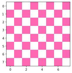
Let’s start with this image of your humble chessboard:

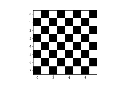
Believe it or not, I just made this using NumPy!

Let’s assume that we have a 8x8 NumPy array named chessboard. Let’s take a peek at its top-most row. This is a row where the left-most pixel is white:

chessboard[0]

array([255,   0, 255,   0, 255,   0, 255,   0], dtype=uint8)

Now let’s look at the second row. This is a row where the left-most pixel is black:

chessboard[1]

array([  0, 255,   0, 255,   0, 255,   0, 255], dtype=uint8)

Each number represents a pixel intensity that ranges from 0 to 255. That is, there are 256 possible values in this colour system. As you might have guessed, 0 here represents black and 255 represents white. Everything in between is a shade of grey.

To make the chessboard, I simply stacked these white and black rows until I got an array of dimensions 8x8 (i.e. 8 rows and 8 columns):

import matplotlib.pyplot as plt
import numpy as np

white_row = np.zeros(8).astype(np.uint8)
black_row = np.zeros(8).astype(np.uint8)
black_row[[1, 3, 5, 7]] = 255
white_row[[0, 2, 4, 6]] = 255

chessboard = np.array([
    white_row,
    black_row,
    white_row,
    black_row,
    white_row,
    black_row,
    white_row,
    black_row,
])

print(chessboard)

[[255   0 255   0 255   0 255   0]
 [  0 255   0 255   0 255   0 255]
 [255   0 255   0 255   0 255   0]
 [  0 255   0 255   0 255   0 255]
 [255   0 255   0 255   0 255   0]
 [  0 255   0 255   0 255   0 255]
 [255   0 255   0 255   0 255   0]
 [  0 255   0 255   0 255   0 255]]

Random side note: If everything between 0 and 255 is a shade of grey in our colour system, what’s up with Fifty Shades of Grey? Let’s ignore that Grey happens to be a person’s name. Why not:

\[256 - \textrm{black pixel} - \textrm{white pixel} = \textrm{254 Shades of Grey?}\]

What do these 254 shades of grey look like, anyway? Let’s create a 16x16 NumPy array, because 16x16 = 256, which happens to be the number of pixel intensities we want to plot.

all_shades = np.reshape(np.arange(256), (16,16))

Let’s plot those poor, neglected shades of grey:

_ = plt.imshow(all_shades, cmap='gray')

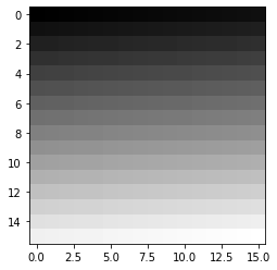
Beautiful, aren’t they?

Enough! ‘Random side note’ over.

What about colour images? Let’s add some volume!

I’m sure most of you have heard of the RGB colour system, where:

• R == 'red',
• G == 'green', and
• B == 'blue'

In a RGB colour image, instead of having a single 8x8 matrix, we now have three:

• a matrix dedicated to intensities of red pixels,
• a matrix dedicated to intensities of green pixels, and
• a matrix dedicated to intensities of blue pixels.

These are called the red, green and blue channels of our RGB image.

Each matrix contains an integer between 0 and 255, where 0 means that the colour in that channel has been effectively turned off, while 255 means that the colour in that channel has been turned on to full.

When we stack these matrices on top of each other, we get a colour image! The RGB system is an example of an additive colour system, where colours are formed by adding pixel intensities across each of the three matrices.

We now know that colour images are three-dimensional volumes. A colour image has:

• a height in pixels,
• a width in pixels, and
• a depth of 3 channels.

Let’s make red, green and blue images!

Firstly, a note on channels-first and channels-last conventions. Our NumPy arrays are of dimensions 3x8x8. That is, our RGB channels come first when describing our array’s dimensions. An alternative convention is the channels-last convention, where channels are listed last in our array’s dimensions (i.e. 8x8x3).

We will be using Matplotlib's imshow function to plot our images. Inspecting the function’s docstring, we see this:

(M, N, 3): an image with RGB values (0-1 float or 0-255 int)…The first two dimensions (M, N) define the rows and columns of the image.

In other words, imshow is expecting a channels-last NumPy array. Don’t worry! We will convert our channels-first images into channels-last by using np.moveaxis to move our channel axis to the end to get a channels-last array:

channels_first = np.zeros((3, 8, 8)).astype(np.uint8)

channels_first.shape

(3, 8, 8)

channels_last = np.moveaxis(channels_first, 0, 2)

channels_last.shape

(8, 8, 3)

Easy, right? Let’s continue.

Let’s turn on all the red pixels. Assuming an RGB ordering, we will set all pixel intensities in our first matrix to the maximum value of 255.

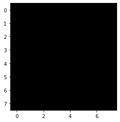
We will start by creating a 3x8x8 array with all pixel intensities turned off (that is, set to zero):

all_pixels_off = np.zeros((3, 8, 8)).astype(np.uint8)

print(all_pixels_off)

[[[0 0 0 0 0 0 0 0]
  [0 0 0 0 0 0 0 0]
  [0 0 0 0 0 0 0 0]
  [0 0 0 0 0 0 0 0]
  [0 0 0 0 0 0 0 0]
  [0 0 0 0 0 0 0 0]
  [0 0 0 0 0 0 0 0]
  [0 0 0 0 0 0 0 0]]

 [[0 0 0 0 0 0 0 0]
  [0 0 0 0 0 0 0 0]
  [0 0 0 0 0 0 0 0]
  [0 0 0 0 0 0 0 0]
  [0 0 0 0 0 0 0 0]
  [0 0 0 0 0 0 0 0]
  [0 0 0 0 0 0 0 0]
  [0 0 0 0 0 0 0 0]]

 [[0 0 0 0 0 0 0 0]
  [0 0 0 0 0 0 0 0]
  [0 0 0 0 0 0 0 0]
  [0 0 0 0 0 0 0 0]
  [0 0 0 0 0 0 0 0]
  [0 0 0 0 0 0 0 0]
  [0 0 0 0 0 0 0 0]
  [0 0 0 0 0 0 0 0]]]

All channel pixels have been turned off. So it makes sense that we get a completely black image:

_ = plt.imshow(np.moveaxis(all_pixels_off, 0, 2))

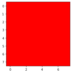
Let’s turn the red pixels onto full:

from copy import deepcopy
red_image = deepcopy(all_pixels_off)
red_image[0, :] = 255

Inspecting the matrix, we see this:

print(red_image)

[[[255 255 255 255 255 255 255 255]
  [255 255 255 255 255 255 255 255]
  [255 255 255 255 255 255 255 255]
  [255 255 255 255 255 255 255 255]
  [255 255 255 255 255 255 255 255]
  [255 255 255 255 255 255 255 255]
  [255 255 255 255 255 255 255 255]
  [255 255 255 255 255 255 255 255]]

 [[  0   0   0   0   0   0   0   0]
  [  0   0   0   0   0   0   0   0]
  [  0   0   0   0   0   0   0   0]
  [  0   0   0   0   0   0   0   0]
  [  0   0   0   0   0   0   0   0]
  [  0   0   0   0   0   0   0   0]
  [  0   0   0   0   0   0   0   0]
  [  0   0   0   0   0   0   0   0]]

 [[  0   0   0   0   0   0   0   0]
  [  0   0   0   0   0   0   0   0]
  [  0   0   0   0   0   0   0   0]
  [  0   0   0   0   0   0   0   0]
  [  0   0   0   0   0   0   0   0]
  [  0   0   0   0   0   0   0   0]
  [  0   0   0   0   0   0   0   0]
  [  0   0   0   0   0   0   0   0]]]

And plotting it, we get this:

_ = plt.imshow(np.moveaxis(red_image, 0, 2))

Repeating for the green pixels:

green_image = deepcopy(all_pixels_off)
green_image[1, :] = 255
print(green_image)

[[[  0   0   0   0   0   0   0   0]
  [  0   0   0   0   0   0   0   0]
  [  0   0   0   0   0   0   0   0]
  [  0   0   0   0   0   0   0   0]
  [  0   0   0   0   0   0   0   0]
  [  0   0   0   0   0   0   0   0]
  [  0   0   0   0   0   0   0   0]
  [  0   0   0   0   0   0   0   0]]

 [[255 255 255 255 255 255 255 255]
  [255 255 255 255 255 255 255 255]
  [255 255 255 255 255 255 255 255]
  [255 255 255 255 255 255 255 255]
  [255 255 255 255 255 255 255 255]
  [255 255 255 255 255 255 255 255]
  [255 255 255 255 255 255 255 255]
  [255 255 255 255 255 255 255 255]]

 [[  0   0   0   0   0   0   0   0]
  [  0   0   0   0   0   0   0   0]
  [  0   0   0   0   0   0   0   0]
  [  0   0   0   0   0   0   0   0]
  [  0   0   0   0   0   0   0   0]
  [  0   0   0   0   0   0   0   0]
  [  0   0   0   0   0   0   0   0]
  [  0   0   0   0   0   0   0   0]]]

_ = plt.imshow(np.moveaxis(green_image, 0, 2))

And again for the blue pixels:

blue_image =  deepcopy(all_pixels_off)
blue_image[2, :] = 255
print(blue_image)

[[[  0   0   0   0   0   0   0   0]
  [  0   0   0   0   0   0   0   0]
  [  0   0   0   0   0   0   0   0]
  [  0   0   0   0   0   0   0   0]
  [  0   0   0   0   0   0   0   0]
  [  0   0   0   0   0   0   0   0]
  [  0   0   0   0   0   0   0   0]
  [  0   0   0   0   0   0   0   0]]

 [[  0   0   0   0   0   0   0   0]
  [  0   0   0   0   0   0   0   0]
  [  0   0   0   0   0   0   0   0]
  [  0   0   0   0   0   0   0   0]
  [  0   0   0   0   0   0   0   0]
  [  0   0   0   0   0   0   0   0]
  [  0   0   0   0   0   0   0   0]
  [  0   0   0   0   0   0   0   0]]

 [[255 255 255 255 255 255 255 255]
  [255 255 255 255 255 255 255 255]
  [255 255 255 255 255 255 255 255]
  [255 255 255 255 255 255 255 255]
  [255 255 255 255 255 255 255 255]
  [255 255 255 255 255 255 255 255]
  [255 255 255 255 255 255 255 255]
  [255 255 255 255 255 255 255 255]]]

_ = plt.imshow(np.moveaxis(blue_image, 0, 2))

What happens if we turn all pixel intensities to full?

Let’s set all pixel intensities in the red, green and blue channels to their maximum values of 255.

all_channels_to_the_max = deepcopy(all_pixels_off)
all_channels_to_the_max[:, :] = 255
print(all_channels_to_the_max)

[[[255 255 255 255 255 255 255 255]
  [255 255 255 255 255 255 255 255]
  [255 255 255 255 255 255 255 255]
  [255 255 255 255 255 255 255 255]
  [255 255 255 255 255 255 255 255]
  [255 255 255 255 255 255 255 255]
  [255 255 255 255 255 255 255 255]
  [255 255 255 255 255 255 255 255]]

 [[255 255 255 255 255 255 255 255]
  [255 255 255 255 255 255 255 255]
  [255 255 255 255 255 255 255 255]
  [255 255 255 255 255 255 255 255]
  [255 255 255 255 255 255 255 255]
  [255 255 255 255 255 255 255 255]
  [255 255 255 255 255 255 255 255]
  [255 255 255 255 255 255 255 255]]

 [[255 255 255 255 255 255 255 255]
  [255 255 255 255 255 255 255 255]
  [255 255 255 255 255 255 255 255]
  [255 255 255 255 255 255 255 255]
  [255 255 255 255 255 255 255 255]
  [255 255 255 255 255 255 255 255]
  [255 255 255 255 255 255 255 255]
  [255 255 255 255 255 255 255 255]]]

_ = plt.imshow(np.moveaxis(all_channels_to_the_max, 0, 2))

We get a completely white image!

How can we get a shade of grey given an RGB image data structure?

You can probably guess what we need to do. Let’s set all pixel intensities to some value between 0 and 255. We will apply the same value across all three matrices:

greyscale = deepcopy(all_pixels_off)
greyscale[:, :] = 150
print(greyscale)

[[[150 150 150 150 150 150 150 150]
  [150 150 150 150 150 150 150 150]
  [150 150 150 150 150 150 150 150]
  [150 150 150 150 150 150 150 150]
  [150 150 150 150 150 150 150 150]
  [150 150 150 150 150 150 150 150]
  [150 150 150 150 150 150 150 150]
  [150 150 150 150 150 150 150 150]]

 [[150 150 150 150 150 150 150 150]
  [150 150 150 150 150 150 150 150]
  [150 150 150 150 150 150 150 150]
  [150 150 150 150 150 150 150 150]
  [150 150 150 150 150 150 150 150]
  [150 150 150 150 150 150 150 150]
  [150 150 150 150 150 150 150 150]
  [150 150 150 150 150 150 150 150]]

 [[150 150 150 150 150 150 150 150]
  [150 150 150 150 150 150 150 150]
  [150 150 150 150 150 150 150 150]
  [150 150 150 150 150 150 150 150]
  [150 150 150 150 150 150 150 150]
  [150 150 150 150 150 150 150 150]
  [150 150 150 150 150 150 150 150]
  [150 150 150 150 150 150 150 150]]]

And plotting it, we get:

_ = plt.imshow(np.moveaxis(greyscale, 0, 2))

Boom! We have ourselves a grey image.

NumPy art: Let’s make a hot pink chessboard!

A quick search tells me that the RBG values for hot pink are these:

red = 255
green = 105
blue = 180

This is what we will do:

• We will make three copies of our original 8x8 chessboard array. One will represent the red channel. Another will represent the green channel. The last one will represent the blue channel.
• We will then alter the pixel intensities of each channel to match the hot pink RBG values, above. We will alter the values of the originally black pixels (i.e. the zeros).
• Once we are done with this, we will create a 3x8x8 array which will represent our chessboard in the RBG colour space.

When we plot the image, we will hopefully see a fabulous, hot pink chessboard. Let’s do it!

First, the copies:

red_channel = deepcopy(chessboard)
green_channel = deepcopy(chessboard)
blue_channel = deepcopy(chessboard)

Next, the pixel values:

red_channel[np.where(red_channel == 0)] = 255
green_channel[np.where(green_channel == 0)] = 105
blue_channel[np.where(blue_channel == 0)] = 180

Let’s create our 3x8x8 array, where the 3 represents our channels:

hot_pink_chessboard = np.array([red_channel, green_channel, blue_channel]).astype(np.uint8)

hot_pink_chessboard

array([[[255, 255, 255, 255, 255, 255, 255, 255],
        [255, 255, 255, 255, 255, 255, 255, 255],
        [255, 255, 255, 255, 255, 255, 255, 255],
        [255, 255, 255, 255, 255, 255, 255, 255],
        [255, 255, 255, 255, 255, 255, 255, 255],
        [255, 255, 255, 255, 255, 255, 255, 255],
        [255, 255, 255, 255, 255, 255, 255, 255],
        [255, 255, 255, 255, 255, 255, 255, 255]],

       [[255, 105, 255, 105, 255, 105, 255, 105],
        [105, 255, 105, 255, 105, 255, 105, 255],
        [255, 105, 255, 105, 255, 105, 255, 105],
        [105, 255, 105, 255, 105, 255, 105, 255],
        [255, 105, 255, 105, 255, 105, 255, 105],
        [105, 255, 105, 255, 105, 255, 105, 255],
        [255, 105, 255, 105, 255, 105, 255, 105],
        [105, 255, 105, 255, 105, 255, 105, 255]],

       [[255, 180, 255, 180, 255, 180, 255, 180],
        [180, 255, 180, 255, 180, 255, 180, 255],
        [255, 180, 255, 180, 255, 180, 255, 180],
        [180, 255, 180, 255, 180, 255, 180, 255],
        [255, 180, 255, 180, 255, 180, 255, 180],
        [180, 255, 180, 255, 180, 255, 180, 255],
        [255, 180, 255, 180, 255, 180, 255, 180],
        [180, 255, 180, 255, 180, 255, 180, 255]]], dtype=uint8)

Now the plotting! Drum roll, please…

_ = plt.imshow(np.moveaxis(hot_pink_chessboard, 0, 2))

Hooray!

Psychedelic cats

Let’s use our knowledge of images to mess with images of my cats, Elsa and Smooshie.

We will use the cv2 package to read our cat images into Python. cv2 can be installed by issuing pip install opencv-python.

import cv2
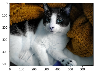
elsa = cv2.imread('./elsa_original.jpg')

Annoyingly, cv2 stores images in a different channel ordering. Instead of RGB, we have BGR. So what we have now is a BGR image. We can see that the colours are a little bit off:

_ = plt.imshow(elsa)

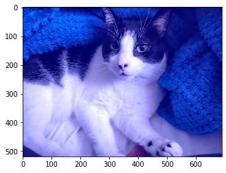
We will now reorder our channels and see if our image looks any better:

elsa = cv2.cvtColor(elsa, cv2.COLOR_BGR2RGB)

_ = plt.imshow(elsa)

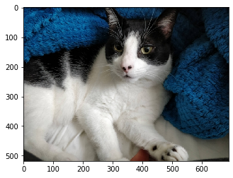
That’s much better!

Let’s increase the pixel intensities of our red channel. Say we want to add 50 to the pixel intensities in our red channel. When using the numpy.uint8 data type, if \(\textrm{current pixel intensity} + 50 > 255\), our pixel intensity wraps around and starts counting from zero. This is an example of integer overflow.

To avoid this, we will be using a suboptimal but quick solution. We will cast our NumPy arrays to the numpy.uint16 data type, which has an upper limit of 65,535. We will add 100 to each pixel intensity. imshow automatically clips the array to have a maximum value of 255 so we will be able to directly plot the image thereafter.

elsa_int16 = elsa.astype(np.int16)
elsa_int16 = np.moveaxis(elsa_int16, 2, 0)

elsa_red = deepcopy(elsa_int16)
elsa_red[0, :] += 100

_ = plt.imshow(np.moveaxis(elsa_red, 0, 2))

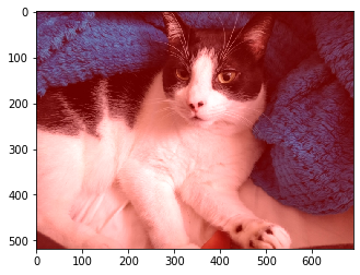
Elsa definitely has a red hue to her!

Let’s repeat with the green channel:

elsa_green = deepcopy(elsa_int16)
elsa_green[1, :] += 100

_ = plt.imshow(np.moveaxis(elsa_green, 0, 2))

Yep, definitely greener! And finally, the blue channel:

elsa_blue = deepcopy(elsa_int16)
elsa_blue[2, :] += 100

_ = plt.imshow(np.moveaxis(elsa_blue, 0, 2))

Yep, definitely blue.

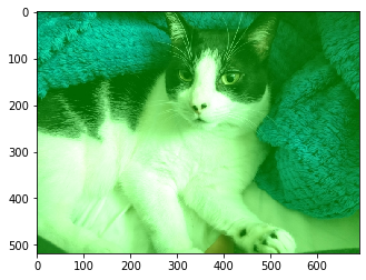
Let’s add arbitrary numbers to each channel to see what we get:

elsa_psychedelic = deepcopy(elsa)
elsa_psychedelic = np.moveaxis(elsa_psychedelic, 2, 0)

elsa_psychedelic[0, :] += 150
elsa_psychedelic[1, :] += 5
elsa_psychedelic[2, :] += 50

_ = plt.imshow(np.moveaxis(elsa_psychedelic, 0, 2))

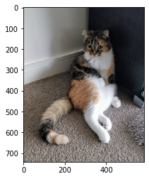
Looking cool, Elsa! What about Smooshie?

smooshie = cv2.imread('./smooshie_original.jpg')
smooshie = cv2.cvtColor(smooshie, cv2.COLOR_BGR2RGB)
_ = plt.imshow(smooshie)

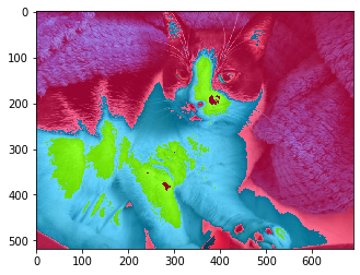
Let’s add some different numbers to Smooshie’s photo:

smooshie_psychedelic = deepcopy(smooshie)
smooshie_psychedelic = np.moveaxis(smooshie_psychedelic, 2, 0)

smooshie_psychedelic[0, :] += 85
smooshie_psychedelic[1, :] += 10
smooshie_psychedelic[2, :] += 175

_ = plt.imshow(np.moveaxis(smooshie_psychedelic, 0, 2))

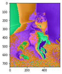
We have ourselves two psychedelic cats!

(Cue ‘Sunshine of Your Love’)

Conclusion

We have learnt how to express images as data that can be manipulated in Python. We made a hot pink chessboard and some psychedelic cat photos along the way!

I hope that this post has given you the foundations that you need to tackle topics such as image kernels which are important in understanding how convolutional neural networks work.

See you next time.

Justin